A/B testing and Fisher's exact test
Marton Trencseni - Tue 03 March 2020 - Data
Introduction
Fisher’s exact test directly computes the same $p$ value as the $\chi^2$ test, without relying on the Central Limit Theorem (CLT) to hold, so it is accurate at low $N$. See the previous post on A/B testing and the Chi-squared test for an introduction to the $\chi^2$ test. The trade-off is that Fisher’s exact test is more computationally intensive, so even at moderate $N$ the direct computation is not feasible. However, Monte Carlo sampling can be used to get estimated results quickly.
The code shown below is up on Github.
Diversion: the Binomial test
The best way to understand Fisher’s test is by a simpler analogue, coin flips. Suppose somebody gives you a coin, and you’re trying to decide whether the coin is fair. If you can flip it a lot of times, you can use a Z-test to decide whether it’s fair or not, because at high $N$, the CLT holds, and the distribution of heads follows a normal distribution.
But, what if you’re only allowed to flip it $N=24$ times and you get $H=18$ heads? This is a low $N$, so the Z-test will not work. But, we can just directly compute the p value by computing $ P(H >= 18 \vee H <= 6) $ assuming the null hypothesis of a fair toin coss. Note that we’re doing a two-tailed test here. $ P(H >= 18 \vee H <= 6) = P(H = 1) + ... + P(H = 6) + P(H = 18) + ... + P(H = 24)$, where $ P(H = k) = {n \choose k} p^k q^{n-k} $, where $p = 0.5, q = 1 - p = 0.5$ in this case from the null hypothesis ($p$ is the probability of heads, $q$ of tails).
What we’re doing here is called the Binomial test. The scipy stats package has a library function:
p = binom_test(18, 24, 0.5)
print('%.3f' % p)
Prints:
0.023
We can calculate this ourselves per the above formula, we just have to be careful with the rounding:
def binomial_test(k, n, p):
    delta = abs(n/2.0 - k)
    lo = floor(n/2.0 - delta)
    hi = ceil(n/2.0 + delta)
    p = 0
    for i in chain(range(0, lo + 1), range(hi, n + 1)):
        p += binom(n, i) * p**i * (1.0 - p)**(n-i)
    return p
This is a direct p value calculation, it works at any $N$. Let’s double-check what we know. According to the CLT, at high $N$ the average ratio of heads will follow a normal distribution, so we can use the Z-test, and it should yield the same result as the direct calculation above:
N = 10*1000
H = 5100 # delta of +1% lift
p = 0.5 # the null hypothesis
raw_data = H * [1] + (N-H) * [0]
print('Binom test p: %.3f' % binom_test(H, N, p))
print('Z-test p:     %.3f' % ztest(x1=raw_data, value=p)[1])
Prints:
Binom test p: 0.047
Z-test p:     0.045
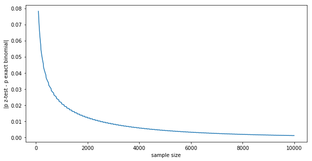
Not quite the same, but pretty close. We can see how the exact binomial and the normal estimated Z-test p values converge thanks to the CLT:
p = 0.5 # the null hypothesis
actual_lift = 0.01
results = []
for N in range(100, 10*1000, 10):
    H = int((p + actual_lift) * N)
    raw_data = H * [1] + (N-H) * [0]
    p_binom = binom_test(H, N, p)
    p_z = ztest(x1=raw_data, value=p)[1]
    p_diff = abs(p_binom - p_z)
    results.append((N, p_diff))

plt.xlabel('sample size')
plt.ylabel('|p z-test - p exact binomial|')
plt.plot([x[0] for x in results], [x[1] for x in results])
plt.show()
The difference goes to zero in the $N \rightarrow \infty $ limit:
Fisher’s exact test
What the binomial test is to the Z-test, Fisher’s exact test is to the $\chi^2$ test. It’s a direct calculation of the p value in case of a $F \times C$ contingency table. Fisher’s exact test is accurate at all $N$s, and the $\chi^2$ test’s p converges to it at high $N$s, similar to the above case.
The null hypothesis is that all funnels have the same conversion event probabilities. Given the $F \times C$ contingency table outcome of an A/B test ($F$ funnels tested, $C$ mutually exclusive conversion events), the calculation of the p value is:
- first, calculate the marginals:
- row marginals: how many users were randomly assigned into each funnel in the A/B test
- column marginals: across the tested funnels, conversion event totals
- given the marginals, what is the probability of the observed outcomes
- for all the ways we can change numbers in the contingency table while keeping the marginals fixed, take the ones that have equal or lower probability then the actual outcome, and add up those probabilities; this is the p value
The trick is, how to calculate the quantity “given the marginals, what is the probability of a specific outcome (numbers in the contingency table that add up to the marginals)”; we need this in both step 2. and 3. For this we have to use the hypergeometric distribution, the distribution for “urn draws”. Let’s reuse the contingency table from the previous post:
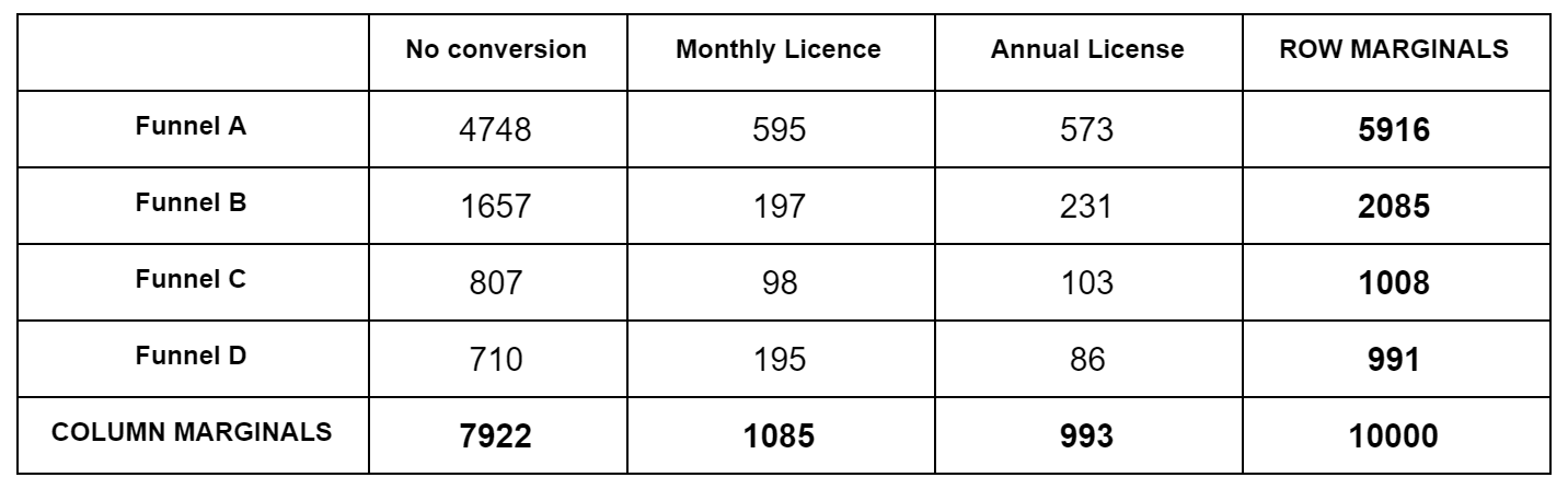
Imagine this: we have a total of $N=10,000$ marbles. Each marble is one of $C=3$ colors (No conversion, Monthly, Annual). There are a total of 7,922 marbles No conversion marbles, 1,085 Monthly conversion marbles, etc. All these marbles are in one big urn. We start drawing marbles; what’s the probability that the first 5,916 drawn will be colored (No conversion, Monthly, Annual) = (4748, 595, 573), irrespective or the order they are drawn? We can break this into two probabilities that we multiply: what is the probability that of 5,916 drawn the colors are (No conversion, Rest) = (4748, 595+573) from an urn that contains (No conversion, Rest) = (7922, 1085+993) marbles, multiplied by, what is the probability that of the rest 595+573=1,168 drawn the colors are (Monthly, Annual) = (595, 573) from an urn that contains (Monthly, Annual) = (1085, 993) marbles. These individual probabilities are given by the hypergeometric probability $P(X=k | N, K, n)$, ie. what is the probability of drawing $k$ red marbles from an urn that contains a total of $N$ marbles, $K$ of which are red, of total $n$ drawn ($k \leq n$). It is $P(X=k | N, K, n) = \frac{ { K \choose k} { N-K \choose n-k } }{ {N \choose n} }$. Then, we go on and calculate the same probabilities in the second row, but keeping in mind that we have already removed (4748, 595, 573) marbles from the urn. The ordering of the rows doesn’t matter.
The formula $P(X=k | N, K, n)$ above is implemented by the scipy hypergeometric probability function hypergeom.pmf, with that we can implement the calculation of the overall probability of a contingency table like:
def hypergeom_probability(observations):
    row_marginals = np.sum(observations, axis=1)
    col_marginals = np.sum(observations, axis=0)
    N = np.sum(observations)
    p = 1
    for i in range(len(observations) - 1):
        for j in range(len(observations[i]) - 1):
            p *= hypergeom.pmf(
              observations[i][j],
              np.sum(col_marginals[j:]),
              col_marginals[j],
              row_marginals[i])
            row_marginals[i] -= observations[i][j]
        col_marginals -= observations[i]
    return p
We can now run an A/B test and whatever the outcome, we can compute the probability of that specific outcome, which will be a very small number:
funnels = [
    [[0.80, 0.10, 0.10], 0.6], # the first vector is the actual outcomes,
    [[0.80, 0.10, 0.10], 0.2], # the second is the traffic split
    [[0.80, 0.10, 0.10], 0.2],
]
N = 50*1000

observations = simulate_abtest(funnels, N)
hypergeom_probability(observations)
But this is not the p value! This is just step 2. To get the p value, per step 3, we have to add up the probabilities for all possible numbers in the contingency table that add up to the marginals, that have lower probability than the actual observations (=are more extreme).
But, even at moderate $N$, there are too many combinations! Instead, what we’ll do is a Monte Carlo (MC) sum. We will randomly sample combinations that satisfy the marginals, and compute the ratio of cases that have lower probability than the given A/B test outcome (= =more extreme outcomes):
def multi_hypergeom_sample(m, colors):
    remaining = np.cumsum(colors[::-1])[::-1]
    result = np.zeros(len(colors), dtype=np.int)
    for i in range(len(colors)-1):
        if m < 1:
            break
        result[i] = np.random.hypergeometric(colors[i], remaining[i+1], m)
        m -= result[i]
    result[-1] = m
    return result

def sample_once(observations):
    row_marginals = np.sum(observations, axis=1)
    col_marginals = np.sum(observations, axis=0)
    sample = np.copy(observations)
    for i in range(len(row_marginals) - 1):
        sample[i] = multi_hypergeom_sample(row_marginals[i], col_marginals)
        col_marginals -= sample[i]
    sample[len(sample) - 1] = col_marginals
    return sample

def fisher_monte_carlo(observations, num_simulations=10*1000):
    p_obs = hypergeom_probability(observations)
    hits = 0
    for _ in range(num_simulations):
        sample = sample_once(observations)
        p_sample = hypergeom_probability(sample)
        if p_sample <= p_obs:
            hits += 1
    return hits/num_simulations
Our implementation above works for arbitrary $F \times C$ contingency tables. The scipy stats library has Fisher’s exact test built in, but it only works for 2x2 tables. Also, remember that we also have the $\chi^2$ test. Let’s compare the three for 2x2 cases:
funnels = [
    [[0.60, 0.40], 0.5], # the first vector is the actual outcomes,
    [[0.60, 0.40], 0.5], # the second is the traffic split
]
N = 100

observations = simulate_abtest(funnels, N)
print(observations)
ch = chi2_contingency(observations, correction=False)
print('chi-squared p = %.3f' % ch[1])
fs = fisher_exact(observations)
print('fishers exact p = %.3f' % fs[1])
fmc = fisher_monte_carlo(observations)
print("""monte carlo p = %.3f""" % fmc)
Prints something like:
[[37. 16.]
 [31. 16.]]
chi-squared p = 0.680
fishers exact p = 0.830
monte carlo p = 0.831
The p value coming from fisher_exact() is exact, the one coming from chi2_contingency() assumes the Central Limit Theorem, while the one coming from our own fisher_monte_carlo() involves a Monte Carlo approximation. Similar to the binomial toin coss example above, let’s see what happens to the differences in $p$ values with increasing $N$, given two funnels and an actual conversion lift of 1%:
base_conversion = 0.5
traffic_split = 0.5
actual_lift = 0.01

results = []
for N in range(100, 20*1000, 200):
    observations = [
        [int(base_conversion * traffic_split * N),
         int((1-base_conversion) * traffic_split * N)],
        [int((base_conversion+actual_lift) * (1-traffic_split) * N),
         int((1-(base_conversion+actual_lift)) * (1-traffic_split) * N)],
    ]
    p_chi2 = chi2_contingency(observations, correction=False)[1]
    p_fish = fisher_exact(observations)[1]
    p_fmc = fisher_monte_carlo(observations, num_simulations=100*1000)
    p_diff_chi2_fish = abs(p_chi2 - p_fish)
    p_diff_chi2_fmc = abs(p_chi2 - p_fmc)
    p_diff_fish_fmc = abs(p_fish - p_fmc)
    results.append((N, p_diff_chi2_fish, p_diff_chi2_fmc, p_diff_fish_fmc))

plt.figure(figsize=(10,5))
plt.xlabel('sample size')
plt.ylabel("""p diff""")
plt.plot([x[0] for x in results], [x[1] for x in results])
plt.plot([x[0] for x in results], [x[2] for x in results])
plt.plot([x[0] for x in results], [x[3] for x in results])
plt.legend([
  '| chi^2 - fisher exact |',
  '| chi^2 - fisher mc |',
  '| fisher exact - fisher mc |'],
  loc='upper right')
plt.show()
The result is:
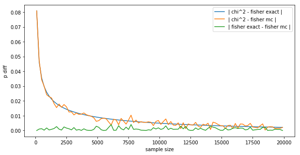
This is a very interesting plot:
- The difference between Fisher’s exact and the MC is wiggling around 0 (green line), not exactly 0 because of the random nature of MC.
- The difference between Fisher’s exact and the $\chi^2$ (blue line) converges to 0 smoothly, like the difference between the z-test and the binomial test in the introduction.
- The difference between the $\chi^2$ and the MC (orange line) follows the blue line, but is a bit more random, again because of the random nature of MC.
- We could get the MC to be smoother by letting it run longer, here it sampled $m=100,000$, we could let it run 10x longer for more smoothness.
This gives us confidence that our MC implementation is correct. However, unlike Fisher’s exact test, and like the $\chi^2$ test, our Monte Carlo version also works on bigger contingency tables:
funnels = [
    [[0.60, 0.20, 0.20], 0.6], # the first vector is the actual outcomes,
    [[0.60, 0.20, 0.20], 0.2], # the second is the traffic split
    [[0.70, 0.15, 0.15], 0.2],
]
N = 1000

observations = simulate_abtest(funnels, N)
print(observations)
ch = chi2_contingency(observations, correction=False)
print('chi-squared p = %.3f' % ch[1])
mcp = fisher_monte_carlo(observations, num_simulations=100*1000)
print("""monte carlo p = %.3f""" % mcp)
Prints something like:
[[368. 113. 112.]
 [126.  45.  55.]
 [125.  26.  30.]]
chi-squared p = 0.076
monte carlo p = 0.078
Conclusion
At this point we have 3 tests we can use for conversion tests: Fisher’s exact, Fisher MC and $\chi^2$. At low $N$, the Fisher ones are more accurate, the exact one (the scipy stats library implementation) only works on 2x2 contingency tables, while our MC one works for any $F \times C$ case. If we let the MC collect enough samples, the two yield the same results numerically. At high $N$, all 3 yield the same results numerically, the simplest thing to do is use the $\chi^2$ test.