A/B testing and networks effects

Introduction

In the previous post I calculated the expected average posts on a social network. The model had 2 components:

• intrinsic: users intrinsically create posts
• network effects: users create more posts if they see their friends’ posts

But, there is actually a third, even more nuanced effect: the strength of the network effect depends on the degree distribution in the network.

The code shown below is up on Github.

Degree dependence of the network effect

Simulations showed that even a weak network effect boosts overall post production significantly. If $c_{int}$ is intrinsic post production, and for each friend's post users create an additional $c_{net}$ post the next day, and on average users have $k$ friends, then in the steady state $c = c_{int} + c \times c_{net} \times k $. Solving this we get $ c = \frac{ c_{int} }{ 1 - c_{net} \times k } $.

In the last post, I used a $U(0, 1)$ random variable to multiply both $c_{int}$ and $c_{net}$. This is not neccessary and just introduces noise, so let’s leave it out. For this post let’s use $c_{int}=1/4$ and $c_{net}=3/200$, with these values $c=1$.

In the above formula, the structure of the graph only appears in the parameter $k$. This is a good first approximation, but it’s not entirely accurate. A more accurate way to think about it is to write $c = c_{int} + c \times f(c_{net}, g) $, where $f$ is some function, and $g$ is the graph ($f=c_{net} \times k$ is our initial approximation). Let's explore this dependence further.

We are using Watts-Strogatz graphs for these experiment, which have a re-wiring randomization parameter $p$. When the Watts-Strogatz graph is constructed, initially a ring graph is created (large diameter) with $k$ edges from each node, and then each edge is randomly re-wired with probability $p$ to get a small-world network (small diameter). If we set $p=0$, the degree distribution of the graph is exactly $k$. As we increase $p$, the degree distribution becomes a gaussian around $k$. Code to visualize this:

Note: some of these simulations take a while to run, so I now use multiprocessing. This makes the code harder to read, but the speed-up is significant.

def mp_degree_distribution(args):
    (n, k, p) = args
    g = connected_watts_strogatz_graph(n, k, p)
    ds = Counter(sorted([d for n, d in g.degree()], reverse=True))
    d, c = zip(*ds.items())
    return p, d, c

n=100*1000
k=50

results = mp_map(
    network_scaling_worker.mp_degree_distribution,
    [(n, k, p/100.0) for p in range(10, 110, 20)])

plt.figure(figsize=(10,5))
plt.xlabel('degree')
plt.ylabel('node count')
for x in results:
    plt.plot(x[1], x[2])
plt.legend(['p=%s' % x[0] for x in results])
plt.show() 

Shows:

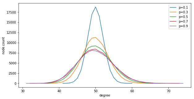
Now comes the interesting bit. Let’s calculate the average post production for a Watts-Strogatz graph for different parameters $(n, p)$, with fixed $k=50$:

def mp_lifts(args):
    (n, k, p, N, T) = args
    g = connected_watts_strogatz_graph(n, k, p).to_directed()
    population_A = set(sample(g.nodes, N))
    stats = compute_stats(g, population_A, T) # see the previous post
    return (args, stats)

ns = [10*1000, 50*1000, 100*1000, 300*1000]
k=50
ps = range(0, 120, 20)
T=50
N=0

results = []
for n in ns:
    print('Running simulations for n=%s...' % n)
    start_time = time.time()
    results.extend(mp_map(
        network_scaling_worker.mp_lifts,
        [(n, k, p/100.0, N, T) for p in ps],
    ))
    elapsed_time = time.time() - start_time
    print('Done! Elapsed %s' % time.strftime("%M:%S", time.gmtime(elapsed_time)))

Shows:

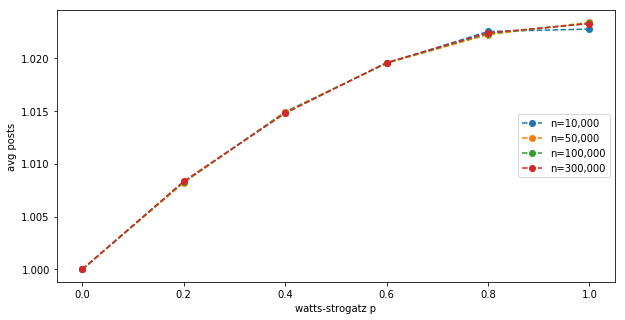
This shows the (third) effect:

• At $p=0$, when all nodes have exactly $k$ neighbours, the mean post production is exactly 1.
• At higher $p$, there is an additional boost to post production, due to some nodes having more neighbours than $k$; and this boost is not canceled by some nodes having less neighbours.
• The maximum boost due to uneven degree distribution is about 2.5% at $p=1$ for $k=50$.
• The effect does not seem to depend on the $n$ network size.

This has implications for A/B testing: when we compute the lift in our simulations, we need to use this adjusted baseline.

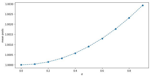
Another way to get a sense for this is: assume half the nodes are have degree $k=50-d$, half have $k=50+d$ after randomization, so the mean is still $k=50$. We can take the original formula $ c = \frac{ c_{int} }{ 1 - c_{net} \times k } $ and make an improved version: $ c(d) = \frac{1}{2} ( \frac{ c_{int} }{ 1 - c_{net} \times (k+d) } + \frac{ c_{int} }{ 1 - c_{net} \times (k-d) } ) $. This is not the exact formula (the experimental result above is concave, and this is convex), but it’s good for intuition:

Initially I suspected the effect is due to the graph diameter decreasing with increasing $p$, so I checked how the mean shortest path depends on $p$ and $n$:

def mp_shortest_paths(args):
    (n, k, p, num_samples) = args
    g = connected_watts_strogatz_graph(n, k, p)
    samples = []
    for _ in range(num_samples):
        st = sample(g.nodes, 2)
        l = nx.shortest_path_length(g, st[0], st[1])
        samples.append(l)
    mean_shortest_path = np.mean(samples)
    return (args, mean_shortest_path)

ns = [10*1000, 50*1000, 100*1000, 300*1000]
k=50
ps = range(0, 120, 20)
num_samples = 1000

results = []
for n in ns:
    print('Running simulations for n=%s...' % n)
    start_time = time.time()
    results.extend(mp_map(
        network_scaling_worker.mp_shortest_paths,
        [(n, k, p/100.0, num_samples) for p in ps],
    ))
    elapsed_time = time.time() - start_time
    print('Done! Elapsed %s' % time.strftime("%M:%S", time.gmtime(elapsed_time)))

Shows:

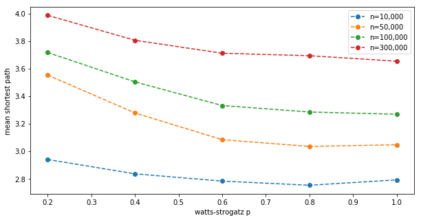
This does not appear to be the reason for the additional boost. The mean shortest path in the graph strongly depends on $n$, as expected, but the effect does not. Intuitively, since all nodes are equal for now (there is no A population producing more content), path length shouldn’t matter.

So, to get more accurate lift readings for our A/B tests, we need to first calculate the correct baseline mean posts for a Watts-Strogatz graph with those $(k, p)$ params (no strong $n$ dependence, experimentally, as we just saw):

n=100*1000
k=50
p=0.1
T=50

g = connected_watts_strogatz_graph(n=n, k=k, p=p).to_directed()
posts = prev_posts = None
for t in range(T):
    posts = step_posts(g, prev_posts)
    prev_posts = posts
baseline_avg_posts = np.mean(list(posts.values()))
print("Correct baseline for a (%s, %s, %s) Watts-Strogatz graph after %s steps = %.4f" % (n, k, p, T, baseline_avg_posts))

Prints:

Correct baseline for a (100000, 50, 0.1) Watts-Strogatz graph after 50 steps = 1.0044

A/B testing

Let’s re-run the A/B test experiment from the last post and calculate the lifts, but compared to the new, corrected baseline. Let’s have an experimental group of $N$ people, whose intrinsic post production $c_{int}$ is lifted by 5%, using both $N=100$ and $N=1,000$:

ns = [5*1000, 10*1000, 50*1000, 100*1000]
k=50
p=0.1
T=50
num_simulations = 50

params = chain(
    prepend(100,  ns),
    prepend(1000, ns),
)

def thread_count(n):
    if n <= 100*1000: return 24
    if n == 200*1000: return 12
    else:             return 8

stats_list = []
if __name__ ==  '__main__':
    for N, n in params:
        print('Running simulations for n=%s...' % n)
        start_time = time.time()
        results = mp_map(
            network_scaling_worker.mp_lifts,
            [(n, k, p, N, T) for _ in range(num_simulations)],
            thread_count(n),
        )
        avg_stats = [np.mean([x[1][i] for x in results]) for i in range(len(results[0][1]))]
        stats_list.append((N, n, avg_stats))
        elapsed_time = time.time() - start_time
        print('Done! Elapsed %s' % time.strftime("%M:%S", time.gmtime(elapsed_time)))

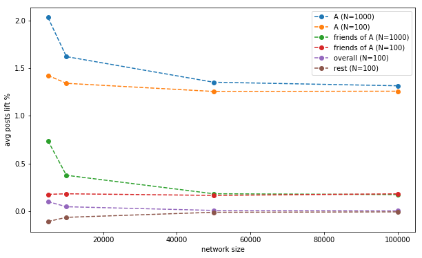
What we expect to see:

• as $N/n$ goes to 0, the rest and overall lifts tend to 0.
• as $N/n$ goes to 1, we expted to see a bigger lift for population A (if $N=n$, we released to 100% and lifted everybody's post production)

Conclusion

A simple toy post production model on a Watts-Strogatz graph shows multiple interesting effects (also see previous post):

• network effect: boosts post production by a significant factor
• degree distribution effect: the network effect boost is a function of the graph's degree distribituion, which for a Watts-Strogatz graph is a function of $p$
• dampening effect: we underestimate the true intrinsic lift of the A/B test, because A’s non-A friends don’t get the intrinsic post production boost, so As don’t get the boost “back” through these edges
• spillover effect: we measure a lift due to the network effect for friends of A, and further down the network, depending on the distance from As
• clustering effect: if the A group is more tightly clustered, we measured a higher lift
• experiment size effect: as $N/n$ goes to 1, the effect size approaches the true effect size