PyTorch Basics: Solving the Ax=b matrix equation with gradient descent

Introduction

PyTorch is my favorite deep learning framework, because it's a hacker's deep learning framework. It’s easier to work with than Tensorflow, which was developed for Google’s internal use-cases and ways of working, which just doesn’t apply to use-cases that are several orders of magnitude smaller (less data, less features, less prediction volume, less people working on it). This is not a PyTorch vs Tensorflow comparison post, for that see this post. There are tons of great tutorials and talks that help people quickly get a deep neural network model up and running with PyTorch. PyTorch comes with standard datasets (like MNIST) and famous models (like Alexnet) out of the box.

Under the hood, PyTorch is computing derivatives of functions, and backpropagating the gradients in a computational graph; this is called autograd. This can also be applied to solve problems that don’t explicitly involve a deep neural network.

To illustrate this, we will show how to solve the standard A x = b matrix equation with PyTorch. This is a good toy problem to show some guts of the framework without involving neural networks.

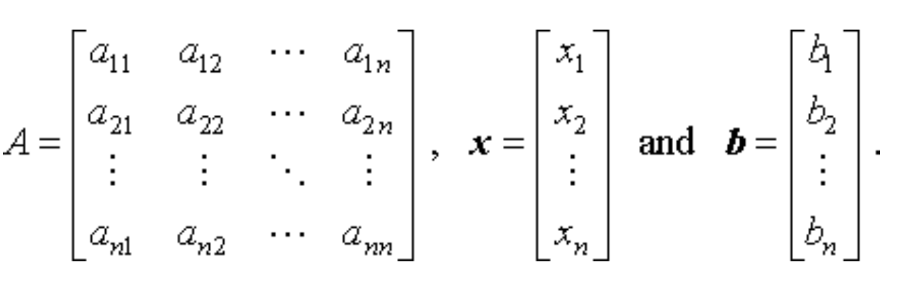
As a reminder, in the A x = b matrix equation, A is a fixed matrix, b is a fixed vector, and we’re looking for vector x such that A x is just the vector b. If A is a 1x1 matrix, then this is just a scalar equation, and x = b / A. Let’s write this as x = A^-1 b, and then this applies to the n x n matrix case as well: the exact solution is to compute the inverse of A, and multiply it by b. (Note: the technical conditions for a solution is det A ≠ 0, I'll ignore this since I'll be using random matrices). Let’s say the solution is x = x_s.

Note: using gradient descent to estimate the solution is not necessary, as the solution can be computed quickly with matrix inversion. We're doing this to understand PyTorch on a toy problem.

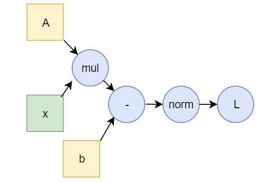
How can we use PyTorch and autograd to solve it? We can use it to approximate the solution: start with some random x₀, compute the vector A x₀ - b, take the norm L = ‖ A x₀ - b ‖, and use gradient descent to find a next, better x₁ vector so that it’s closer to the real solution x_s. They key idea is that for x=x_s, the norm L = ‖ A x_s - b ‖ = 0, it vanishes. So we want to minimize L. This L is called the loss function in such optimization problems.

Let’s start with the standard L2 norm:

This will result in a parabolic loss function, where we will converge to the minimum.

Code

This is what the PyTorch code for setting up A, x and b looks like. We initialize A and b to random:

We set requires_grad to False for A and b. These are constants in this scenario, their gradient is zero. x is the variable which we will compute gradients for, so we set requires_grad = True.

We then tell PyTorch to do a backward pass and compute the gradients:

At this point, PyTorch will have computed the gradient for x, stored in x.grad.data. What this means is “adjust x in this direction, by this much, to decrease the loss function, given what x is right now”. Now we just need to introduce a step size to control our speed of descent, and actually adjust x:

Almost done. We just need to set step_size, put this in a for loop, and figure out when to stop it:

Let’s stop it when the loss is smaller than stop_loss, and put an upper bound on the number of iterations. Putting it all together:

It’s a good exercise to play around with this. Set a specific A and b, print things out, try other dimensions, use numpy to get the inverse and compare the solutions, etc.

Discussion

How is this related to neural networks?
In a fully connected (FC) layer, each input is multiplied by a weight to get the next's layer values. Putting the weights together, they form a matrix (tensor), which is multiplied by the input activations, just like A x. In real neural networks, non-linearity is introduced at each node, eg. a ReLu function; we don't have that, this is a linear problem. Note that in real machine learning scenarios, the loss function (potential surface) is in a very high dimensional space and has several minima; the goal is not to find the global optimum (which is untractable), just a good enough local one (that gets the job done).

How do we know what step_size should be? How do we know when to stop?
In this case, because the loss function we’re optimizing is quadratic, we can get away with a fixed step size, as the gradient will get smaller as we approach the optimum (the solution). In more complicated deep neural network scenarios (where the step size is called the learning rate), there are strategies on how to gradually decay the step size. In general, if the step size is too small, we waste a lot of time far away from the solution. If it’s too big, we jump around the optimum and it may never converge. See also Learning Rate Schedules and Adaptive Learning Rate Methods for Deep Learning.

What should the stopping condition be?
In this toy example, the step_size is set smaller than stop_loss, so it can converge on the optimum below the accepted loss. If you would set the stop_loss to be much smaller than the step size, you will see that it never stops, it will jump around the optimum (left side of above picture).

What exactly is the quantity x.grad.data?
It's the gradient of the loss function we called backward() on, with respect to the variable, in this case x. So in the dim=1 case it’s just dL/dx. Note that since x is the only independent variable here, the partial derivative is the total derivative. If we had multiple independent variables, we'd have to add the partial derivates to get the total derivative.

What if we use the L1 norm as the loss function?
To use the L1 norm, set p=1 in the code. The L1 norm in dim=1 is the abs() function, so it’s derivative is piecewise constant. In this case the slope is +- ‖A ‖.

This is “less nice” than the L2 norm for this simple case, because the gradient doesn’t vanish as the solution approaches the optimum. The solution is more likely to overshoot the optimum and oscillate.

What happens if we run this on the GPU?
To turn on the GPU, put this line at the top:

On my computer, this is significantly slower on the GPU than the CPU, because copying such a small problem to the GPU on each iteration creates a time overhead which is not worth it. This toy example is too small to demonstrate how GPUs speed up deep learning.