Running multiple A/B tests in parallel

Introduction

Suppose we have N=10,000 users and want to run 2 A/B test experiments, $E_1$ and $E_2$, both of which are trying to move the same metric. In this post I will assume the metric we are trying to move is timespent per user (or something like it, a number assigned to each user). The same logic also applies to conversions, but timespents are a better illustration of the concepts.

It is a common misconception that when running two experiments, we have to split our users between the two experiments, so each experiment will have 50,000 users in it, and each bucket will have 2,500 users in it (A in $E_1$, B in $E_1$, A in $E_2$, B in $E_2$). The cause of this misconception is the belief that if a user is in both experiments, then we cannot tell which experiment led to the user spending more time.

At face value, this is an error in statistical reasoning. We don’t really care why an individual user spent more or less time with the product, what we care about is the average timespent between A and B. As long as that measurement is accurate, individual users’ being influenced by multiple experiments is irrelevant. Accurate here means that we would measure the same thing (statistically) if we were running only one A/B test.

Having said that, there are cases when running multiple tests on the same user leads to statistical errors: this happens if the experiments interact. In other words, if we assume that run by itself $E_1$ lifts by X, and $E_2$ lifts by Y, and if we run both than the lift is X+Y, then we're fine. But if the effects interact with each other, in which case the combined lift is something else (eg. X+Y/2, because the presence of X suppresses Y), then we cannot run them in parallel. This happens if eg. the experiments are making UI changes to the same dialog.

If the experiments are independent, there is in fact no need to limit the sample sizes, both experiments can run on all 100,000 users, in parallel.

The code shown below is up on Github.

Modeling the experiments

To understand why parallel experiments work, let’s remember how an A/B test is modeled in our simulations: each user is represented by a independent random variable (RV). Independent, because we assume users don’t affect each other (so, we’re not in a social network setting here), and it’s a random variable because individual user outcomes are random. In this post, like before, I will use an exponential distribution to model timespents. The exponential distribution has one parameter $\mu$, which works out to be the mean. I will assume that by default, users have $\mu=1$.

In our timespent simulations, when we say that an A/B test is actually working, we model this by increasing the $\mu$ parameter for the user’s random variable. In the end, we will sample the random variable, so the actual outcome can be any timespent $t>0$, but on average, users with lifted parameters will have higher timespents. This is the key: in an A/B test, we don’t care about individual user’s outcomes, since they are statistically random anyway, we care about measuring accurate average lifts between groups of users.

Visualizing one A/B test

There is an easy visual way to understand why parallel A/B tests work. Before we look at the parallel cases, as a starting point, let’s look at the simple case of just one experiment. We can use code like in the previous posts for this:

N=10*1000
funnels = [
    [0.00, 0.5],
    [1.00, 0.5],
]
timespent_params = defaultdict(lambda: 1.0)
timespents = {}

funnel_assignment = simulate_abtest(funnels, N, timespent_params, force_equal=True)

for i, param in timespent_params.items():
    timespents[i] = expon(param).rvs(size=1)[0]

What this code is doing: there are $N=10,000$ users, we will split them evenly between A and B funnels in the experiment (per funnels, 2nd column). Each user is modeled by an exponential random variable's parameter (timespent_params, which has default parameter 1). The function simulate_abtest() assigns each user into A or B, it returns this assignment into funnel_assignment. Further, it adjusts the timespent_params, by increasing the RV’s parameter for users in the B bucket by 1, leaving As alone (per funnels, 1st column). The final for loop samples the exponential distributions and stores the actual timespent values per user in timespents.

We can visualize the outcome of this experiment by drawing both the parameters and the actual timespents of each user. Since there are $N=10,000$ users, we can do so on a 100x100 image. The left side shows the parameters ($\mu=1$ or $\mu=2$), the right side shows the actual, sampled timespents.

Let’s change our visualization a little bit: let’s make it so we draw the A bucket users on top, and the B bucket users on the bottom:

This nicely shows us what’s going on. On the left side, we can see that the random variables for A and B have different values. On the right side, we can see that after sampling, the difference is still discernible with the naked eye. Note that the two left and two right sides are showing the same values, only arranged differently.

Two A/B tests in parallel

Now let’s run 2 A/B tests in parallel. In both cases, A leaves the RV’s parameter alone. But for $E_1$, we lift it to $\mu=2$, for $E_2$ we lift it to $\mu=3$. Users are in both A/B tests, and they are assigned into A and B buckets randomly, independently in the two experiments:

N = 10*1000
num_tests = 2
base_lift = 1
timespent_params = defaultdict(lambda: 1.0)
timespents = {}
funnel_assignments = []
for test in range(num_tests):
    funnels = [
        [0,                  0.5],
        [(test+1)*base_lift, 0.5],
    ]
    funnel_assignment = simulate_abtest(funnels, N, timespent_params)
    funnel_assignments.append(funnel_assignment)

for i, param in timespent_params.items():
    timespents[i] = expon(param).rvs(size=1)[0]

Note that we call simulate_abtest() in a loop, for each experiment. Let’s visualize the outcome here: we expect that the parameter image will have 4 colors, corresponding to whether a user ended up in AA ($\mu=1$), AB ($\mu=2$) BA ($\mu=3$) or BB ($\mu=4$):

The left side image in fact has 4 colors. After random sampling, the right side looks just as random as in the single A/B test case. Now let’s do the same trick as before, and draw the image so that As are on top, and Bs are on the bottom. We can pick whether we do this for $E_1$ or $E_2$, we will see the same thing, here I'm doing it for $E_2$'s A and B:

Note again that these are the same exact values as above, only reordered. We can see that on the left side, there are 2 possible parameters on each side (the A and B variations from the other experiment). And on the right side we can see that even though the other experiment is also running, we can clearly tell apart the average value between top (A) and bottom (B).

After visualization, we can also numerically see this:

for test, funnel_assignment in enumerate(funnel_assignments):
    ps, ts = [[], []], [[], []]
    for i, which_funnel in enumerate(funnel_assignment):
        ts[which_funnel].append(timespents[i])
        ps[which_funnel].append(timespent_params[i])
    ps_means, ts_means = [np.mean(x) for x in ps], [np.mean(x) for x in ts]
    p = CompareMeans.from_data(ts[1], ts[0]).ztest_ind(alternative='larger', usevar='unequal')[1]
    print('test '%02d', experiment lift=%.4f, blended parameter lift=%.4f, measured lift=%.4f, p-value=%.4f'
          % (test, (test+1)*base_lift, ps_means[1]-ps_means[0], ts_means[1]-ts_means[0], p))

Prints something like:

test 00, experiment lift=1.0000, blended parameter lift=0.9700, measured lift=0.9634, p-value=0.0000
test 01, experiment lift=2.0000, blended parameter lift=1.9850, measured lift=1.9924, p-value=0.0000

In the first test, we lifted by 1. Because of the other test also running and changing the random variable parameters, on average our random variable parameters were shifted by 0.97 (instead of 1). After sampling, the actual lift was 0.96. And at this sample size, this lift had a very low p-value (since it’s a doubling, it’s easy to measure). And in the next row, we can see the second A/B test, which is also easily measureable.

Multiple A/B tests in parallel

Maybe this only worked because there were only 2 experiments, and we lifted the RV’s parameter so aggressively (doubling, tripling). Let’s see what happens if we run 11 in parallel, with a $\mu$ lift of 0, 0.1, 0.2 ... 1.0 (so the first one doesn’t work, the last one doubles). The numeric outcomes:

test 00, experiment lift=0.0000, blended parameter lift=0.0605, measured lift=0.0656, p-value=0.0101
test 01, experiment lift=0.1000, blended parameter lift=0.1168, measured lift=0.1027, p-value=0.0001
test 02, experiment lift=0.2000, blended parameter lift=0.2122, measured lift=0.1929, p-value=0.0000
test 03, experiment lift=0.3000, blended parameter lift=0.3125, measured lift=0.3113, p-value=0.0000
test 04, experiment lift=0.4000, blended parameter lift=0.4011, measured lift=0.4153, p-value=0.0000
test 05, experiment lift=0.5000, blended parameter lift=0.5037, measured lift=0.5526, p-value=0.0000
test 06, experiment lift=0.6000, blended parameter lift=0.6013, measured lift=0.5849, p-value=0.0000
test 07, experiment lift=0.7000, blended parameter lift=0.6867, measured lift=0.6740, p-value=0.0000
test 08, experiment lift=0.8000, blended parameter lift=0.8124, measured lift=0.8005, p-value=0.0000
test 09, experiment lift=0.9000, blended parameter lift=0.8973, measured lift=0.8763, p-value=0.0000
test 10, experiment lift=1.0000, blended parameter lift=1.0157, measured lift=1.0209, p-value=0.0000

It’s still pretty good. Let’s visualize the middle one, where $\mu$ is lifted by 0.5:

We can see that on the left, because there are so many A/B tests in play, the RV parameters also look random, but we can still see the difference, also in the sampled timespents on the right side.

Monte Carlo simulations to estimate variance of parallel A/B tests

In the above case, for the 7th test, the true experiment lift was 0.7000, but due to the presence of other A/B tests, the blended parameter lift between the two buckets (left side on the images) was 0.6867. Let’s use Monte Carlo simulations to quantify how much of a variance we can expect, as a function on $N$. Let’s run a scenario where we’re running 7 A/B tests at the same time, with lifts of [0, 0.01, 0.02, 0.03, 0.04, 0.05, 0.10] on different $N$ population sizes [10*1000, 20*1000, 30*1000, 40*1000, 50*1000, 100*1000, 200*1000, 1000*1000]. Let's run each scenario 100 times, and compute means and variances for average parameter lift and actual measured lift.

First, the average parameter lifts, with errors to show the variance:

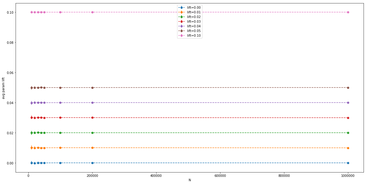
We can see that even at low N, the average parameter lifts are pretty close to the intended experimental lift. The variance is so small, we can barely see it. Let’s zoom in on the orange line:

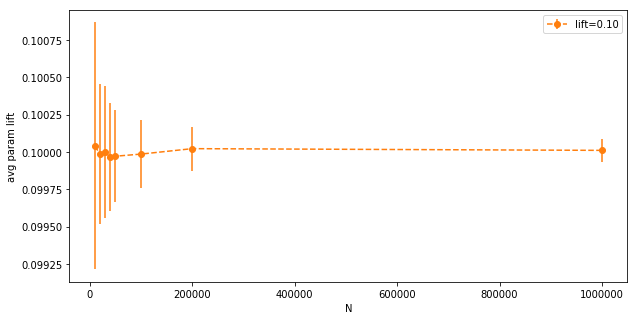
The variance goes down with $N$ as expected, but even at $N=10,000$ it’s very low (notice the y-axis). Now the same for actual measured lifts (after the random variables are sampled):

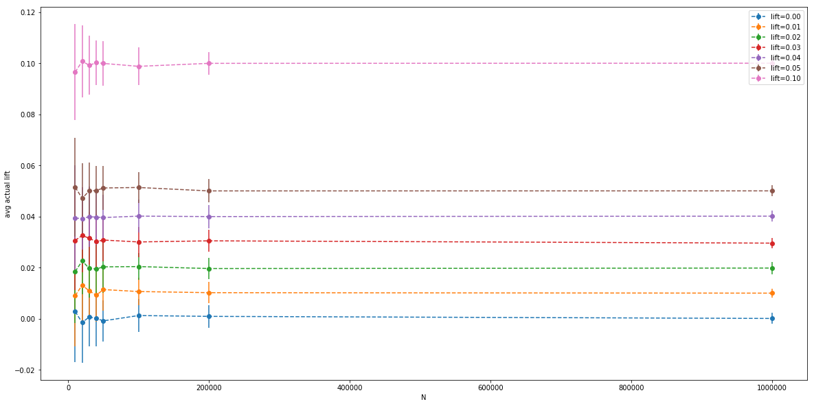
Here we have bigger error bars, it’s hard to see what’s going on. Let’s look at the orange bar again:

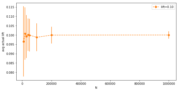
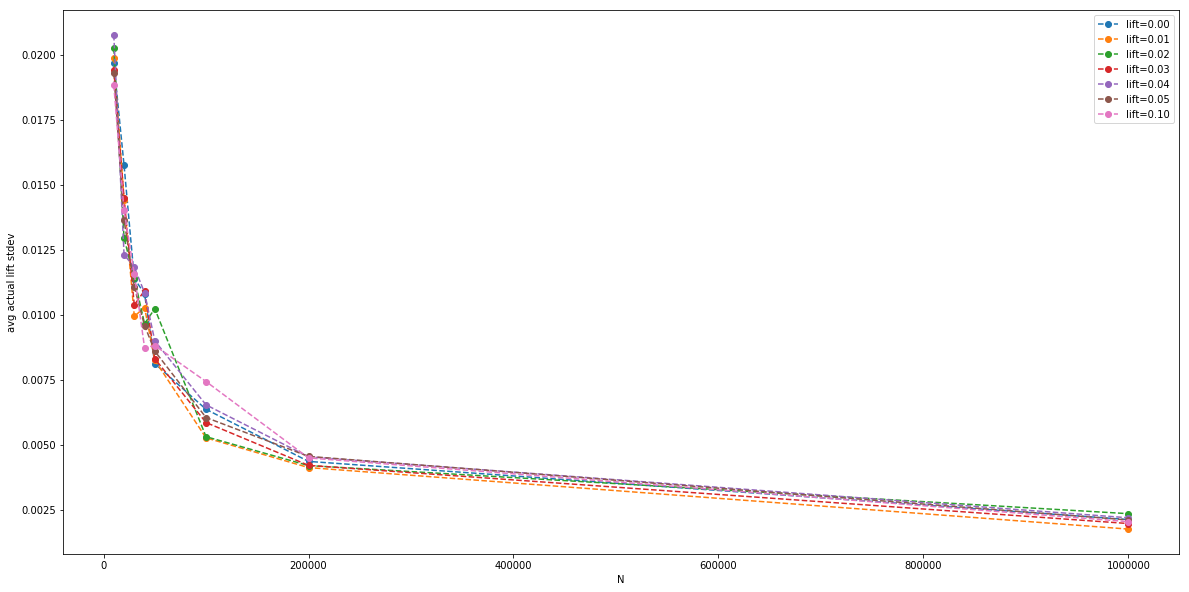
The magnitude of the standard deviation (the error bar), plotted by itself:

Finally, we can plot the average measured p value (with a Z-test), for each parallel A/B test, for each $N$:

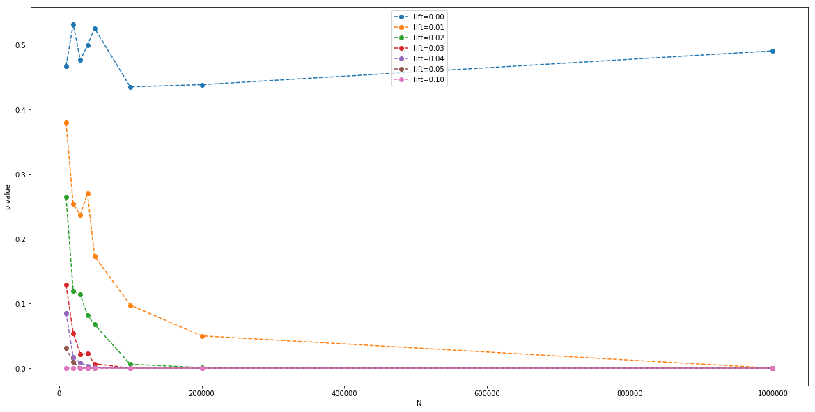
This is essentially a clue to the sample size $N$ we need to be able to detect the signal at a given $\alpha$ critical value of p.

Per experiment random user id

As these Monte Carlo simulations show, it is possible to run multiple A/B tests at once, across the whole population, on the same outcome metric, and still measure the experimental lift accurately, assuming the experiments are independent.

It is only necessary to randomize the users between the funnels A and B (and C...) for each experiment independently of the other experiments. A simple solution for this is to have a once randomly generated test_seed for each experiment that is stored and constant throughout the experiment (like 90bb5357 for experiment $E_1$, a5f50c2b for experiment $E_2$, and so on), combine these with a per user id (like user_id, or cookie_id) to get a per experiment random number, that is fixed for the user (so when the user comes back, we compute the same random number), and then modulo that to the number of funnels we have to decide whether to put the user into A or B in each experiment (so if the user returns, she goes back to the same bucket):

def funnel_user(base_traffic_split, test_seed, user_id):
    test_id = hashlib.md5(test_seed.encode('ascii') + str(user_id).encode('ascii')).hexdigest()
    bits = bin(int(test_id, 16))[3:]
    r = sum([int(bit)*(0.5**(i+1)) for i, bit in enumerate(bits)])
    if r < base_traffic_split:
        return 'A'
    else:
        return 'B'

Conclusion

By randomizing user assignments into A/B test experiments, it is possible to run multiple A/B tests at once and measure accurate lifts on the same metric, assuming the experiments are independent.