Using simulated self-play to solve all OpenAI Gym classic control problems with Pytorch

Introduction

In a previous blog post, I applied plain vanilla Reinforcement Learning policy gradient to solve the CartPole OpenAI gym classic control problem. In the subsequent blog post, I generalized that code (in a software engineering sense) and applied it to all classic control problems; the only "trick" was to quantize the applied action for the continuous problems to convert them to discrete problems. It was able to solve CartPole and Acrobot, but failed on Pendulum and MountainCar (the failure was unrelated to the discretization). I described the problem that I saw examining the numerics at the end of the post:

.. the loss function is structured like loss := -1 * sum(reward x log(probability of action taken)), where the log(probability of action taken) is negative, so the overall expression is positive, assuming the reward is positive. In this case, making the loss 0 would be a global minimum. This can happen if the optimizer sets the probabilities of an arbitrary sub-optimal policy to one, hence making the log(probability) zero, making the entire loss function go to zero, even though the solution is actually "random".

Simulated self-play

It occured to me that this sort of problem wouldn’t occur when using RL for Chess or Go, since in that case, the agent plays itself, and the winner would get a +1 reward, the loser a -1 reward. This means that gradient descent can’t converge on a bad solution by just adjusting the weights so that the probability of an arbitrary action becomes 1, because this gets supressed by the -1 reward parts in the loss function.

It then occured to me that it’s easy to simulate this setup with any game: let the agent play games, and once finished, pair the games, and the one with the higher episode reward (as set by the original rules of the game) is the winner, the other the loser. Overwrite the original reward, and simply use +1 for all actions taken by the winner, and -1 for all actions taken by the loser. In actual implementation, there is no need to actually pair: it’s easier to just play N games, sort the games by overall reward, and treat the lower half as losers and give them -1 rewards, and the upper half as winners and give them +1 rewards. N should be chosen to control variance, I used N=100 here.

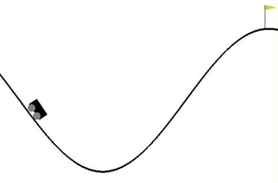
The only "hack" necessary to make this work is on the MountainCar-v0 problem: the way the default reward returned by OpenAI Gym is structured, initially it returns a constant -200 (-1 for each timestep the agent doesn't reach the top of the hill, with 200 timesteps per episode). So with this default reward structure, this approach would fail, because the initial totally random agent has no way of knowing which way to proceed, as all runs return a constant -200 (min=median=avg=max=-200). To make this approach work, I defined a custom reward function, which is simply the maximum x-coordinate that the agent reaches, and set the solved reward threshold at 0.5, which is the position of the flag at the top of the hill.

Coding it up

The code is very similar to the previous solutions. The ipython notebook is up on Github. The main change is in the main training loop, which collects episode results, splits them into winners and losers, and computes the custom loss function based on that:

def train_solve_self_play(env_desc, model=None, num_epochs=5000, num_episodes=100, eps_non_greedy=0.0):
    print('Doing %s' % env_desc.name)
    env = gym.make(env_desc.name)
    input_length, output_length = in_out_length(env)
    if env_desc.output_quantization_levels is not None:
        output_length *= env_desc.output_quantization_levels
    if model is None:
        model = env_desc.model_class(input_length, output_length)
    if env_desc.learning_rate != None:
        lr = env_desc.learning_rate
    else:
        lr = 0.01
    optimizer = optim.Adam(model.parameters(), lr=lr)
    for epoch in range(num_epochs):
        games = play_games(env_desc, env, model, num_episodes, eps_non_greedy)
        games.sort(key=lambda x: x[0]) # sorts by first key, the reward
        losses = games[:int(num_episodes/2)]
        wins = games[int(num_episodes/2):]
        sum_loss = 0
        for game in losses:
            probs = game[1]
            sum_loss += compute_loss(probs, [-1] * len(probs)) # losers get -1 reward for all actions taken
        for game in wins:
            probs = game[1]
            sum_loss += compute_loss(probs, [+1] * len(probs)) # winners get +1 reward for all actions taken
        optimizer.zero_grad()
        sum_loss.backward()
        optimizer.step()
        evaluation_rewards = []
        for _ in range(10):
            reward, _, _ = play_one_game(env_desc, env, model, eps_non_greedy=0.0, policy_func=select_action_from_policy_best)
            evaluation_rewards.append(reward)
        mean_reward = mean(evaluation_rewards)
        print('%d: min=%.2f median=%.2f max=%.2f eval=%.2f' % (epoch, games[0][0], games[int(num_episodes/2)][0], games[-1][0], mean_reward))
        if mean_reward >= reward_threshold(env, env_desc):
            print('Solved!')
            return model
    print('Failed!')
    return model

Results and discussion

This approach solves all the classic control problems from OpenAI Gym. I find it intellectually rewarding to adjust a simple, generic solution so it works across problems. Caveats of this approach are:

• As mentioned above, I had to adjust the reward structure for MountainCar so the training loop is able to tell apart better from worse runs (winners/losers).
• This approach still assumes a discrete action space, which means continuous problems like Pendulum had to be discretized. This would not work or would be very inefficient for higher dimensional action spaces.
• Although this approach works, it's quite slow: in each epoch, 100 games are played; for the simple games like CartPole about 100 epochs are enough, but for MountainCar about 2,000 epochs (so a total of 2,000,000 games played) are needed; other RL methods can find solutions to these simple problems using orders of magnitude less playing time.
• I played around with off-policy learning; this would mean that in epsilon percent of cases, the agent does not pick the action based on the current policy distribution, but totally randomly (ie. uniform); this introduces more random exploration (and noise) into the training process; in the end, this was not needed here.
• As before, I used the Adam optimizer for all problems; I had to adjust learning rate to 0.001 for MountainCar, the default 0.01 worked for the other environments.
• This approach is still naive because it evenly splits each epoch's N games on the median into two equal sets of winners and losers. As the agent approaches a good solution (and the [min, max] range of rewards in the pool of N games becomes tighter and better), this strategy becomes less effective, because good runs are classified as a loss, and the decisions taken are penalized (-1 reward). Similar to adjusting the learning rate, it would be more sophisticated to adjust the ratio of winners and losers as the solution approaches the reward theshold (but I didn't implement that here).