YOLO object detection architecture

Marton Trencseni - Sat 10 July 2021 - Data

Introduction

In the previous post I conducted simple experiments using YOLOv5. I checked how the model responds to rotation, scaling, stretching and blurring, and found that it's reasonably robust against these transformations. I briefly touched on the architecture in the Limitations section of the post:

There is also a local maximum of objects that it can detect, due to the architecture of the neural network. So if there is a large image, with a smaller section containing 100s of objects to be detected, the user will run into this local maximum constraint.

Here I will try to explain the architecture in more detail:

input-output considerations of the neural network
bounding boxes
loss function
training algorithm

Sources:

Input-output considerations of the neural network

Let's zoom out for a moment and think about object detection as an input-output problem. Let's assume the input image is is W pixels wide and H pixels high. If it's grayscale, it can be encoded as a W x H matrix of floats between 0 and 1 representing pixel intensities. If it's an RGB image, it's a 3 channel tensor, 3 x W x H, each layer encoding one color intensity. But, what about the output?

Ideally, the output should be a list of variable length, like:

object 1: confidence Z1, center X1, center Y1, width Q1, height T1, class C1 (like car, dog, cat)
object 2: confidence Z2, center X2, center Y2, width Q2, height T2, class C2
and so on, depending on how many objects are on the image...

However, neural networks cannot return a variable number of outputs. The output of a neural network, like the input, is a tensor, ie. a block of float values.

Notice that each object's information (confidence Z, center X, center Y, width Q, height T, class C) can easily be encoded as a vector, with each value between 0 and 1:

confidence as a probability
center X / image width W is a value between 0 and 1
center Y / image height H is a value between 0 and 1
object width Q / image width W is a value between 0 and 1
object height T / image height H is a value between 0 and 1
each C class gets its own float between 0 and 1, encoding the probability of the object belonging to that class (sum to 1)

So if we have a total of C classes, each detection can be encoded in a vector of 5 + C floats.

One thing we could do is set an M maximum number of objects the network can detect, like M=100 or M=1000, and have the output of the network be a tensor (matrix) of dimensions M x (5 + C), each row encoding a possible object detection. This sounds pretty simple, and similar to the limitations of this scheme, YOLO also has a global limit on number of objects. However, this is not how YOLO works.

The problem with the simple scheme above is that it would be hard to train. Imagine a training image which contains 5 cars. Which of the M rows in the output tensor do we want to give us the detection? There's a danger that certain rows get specialized, so it's always detecting cars of dogs, or detecting objects in certain regions. Then, during usage, if the input image has some other configuration, for example all cars (M cars), then some of the output rows won't be useful.

So YOLO puts a simple twist on the above scheme. It divides the image into an S x S regions, and each region is its own detector. Each region is responsible for detecting images whose bounding box is centered in that region. As before, tensors have to be of a fixed size, so each region can detect up to B objects. This way, the global maximum of objects that can be detected is S x S x B. This way, it's more clear which row is responsible for detecting which object, although there is still ambiguity, but it's greatly reduced, from S x S x B to B. In principle, by increasing S, B could be set to 1, but this is not the case:

in the original YOLOv1 architecture, S = 7 and B = 2, so a total of 7 x 7 x 2 = 98 objects can be detected. C = 20 classes of objects can be detected.
in YOLOv2, S = 13, B = 9.
in later YOLO versions, all these parameters have increased to larger numbers, and can be changed if you train your own network (S, B, C classes)

The center floats are normalized to the region dimensions, so (0, 0) corresponds to the top left corner of the region (not the entire image), (0.5, 0.5) corresponds to the center of the region, and so on.

One more change is that YOLOv1 does not detect a class for each object, it detects a class for each region. So each region can detect B objects, but each region only has one set of C floats for detecting the classes, so the B objects are all of the same class. So in the end, the output tensor of YOLOv1 is S x S x (B x 5 + C) floats. Later, in YOLOv2 this limitation has been removed, and each detection has its own class, making the output tensor S x S x (B x (5 + C)).

Note that the price we pay with this architecture is that if an input image has big blank regions, and lots of small objects clustered in a small region, the network will miss a lot of them due to the local B limit. This is what the quote from the last post was referring to.

One final step is pruning the output. Since a neural network is a "numerical beast", when using the model in production, all output floats will be non-zero, even though there is nothing there. To get rid of this noise, YOLO cuts off object detection confidence at 0.3, so anything less than 0.3 is thrown out as a non-detection.

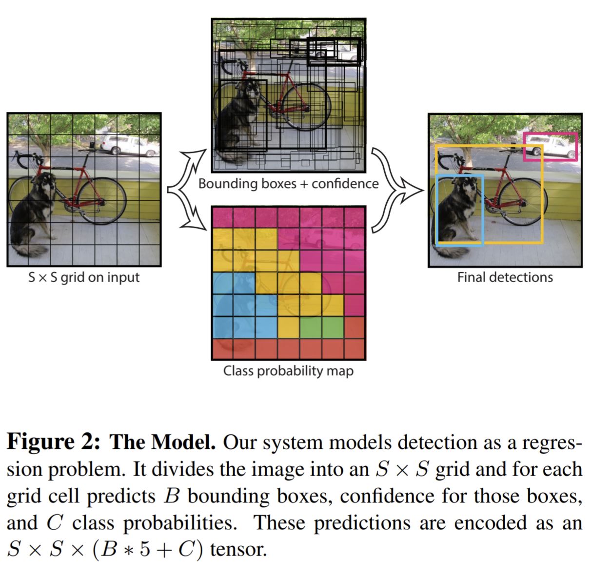
The image above is from the original YOLO paper. Note how each region correspnds to one class (depicted by the colors). This was changed in YOLOv2. The top image shows all 98 bounding boxes, the right side shows the 3 where confidence was higher than 0.3.

Loss function and bounding box scoring during training

Imagine we're training the neural network described above. One data point in the training set is an input picture, along with a set of objects that are on the picture. Each object has a bounding box (center X, center Y, width Q , height T and class C). Suppose we then run this through the neural network. Given the architecture of the network, there is one specific region which contains the center coordinates, which has B detection boxes. So we want that region to detect the box. However, it's possible that:

multiple boxes (of the B) in that region start "finding" the object
boxes in other regions also "find" the object (with shifted bounding boxes)

The question is, how do we "score" these detections, to force the neural network to learn to detect each object once, and in the appropriate region only? In a neural network, this scoring happens through the loss function, so we have to encode our logic / intention in the loss function.

The way the YOLO loss function is set up, detections outside the correct region are deemed incorrect and ignored (zero multiplier in the loss function). Inside the correct region, the detector with the highest overlap gets scored, the rest is ignored (zero multiplier in the loss function). Another trick is to "tell" the loss function that errors in bounding box width and height matter more if the bounding box itself is small (ie. a 10 pixel width error in a 20 pixel wide box matters more than a 10 pixel width error in a 200 pixel wide box). This is accomplished by square-rooting the widths. The overall loss function from YOLOv1 is of a quasi $ L^2$ form:

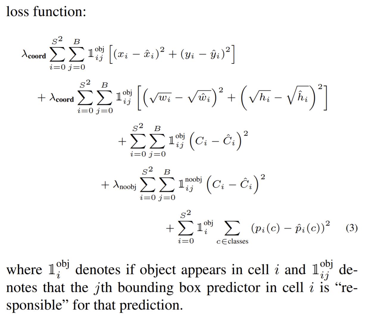
The $ \lambda $ multipliers are set to balance between localization and classification error.

Training method

There are 2 main points about the training method I will point out:

The CNN portion on the deep neural network is pre-trained on ImageNet classification, so it already has some "memory" about what features to pick up. Obviously, it can also be trained on other datasets for other use-cases.
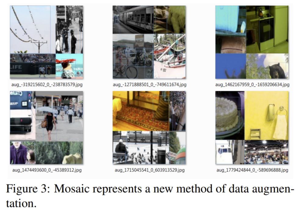
The (C)NNs are not naturally resistant to rotation, scaling, stretching and blurring. Also, they may pick up spurious features, such as a toothbrush always occuring near a face. To make the model more general, the training includes rotation, scaling, blurring, superimposing different parts of images, and so on. Starting in YOLOv4, images are also "mosaiced" together to make the detection less context-dependent.

Conclusion

The YOLO models are deep neural networks, so they're fundamentally black boxes. Like all neural networks, as of today they are more art than science. We don't exactly know why one thing works better than the other. The field is very experimental, and when something works, others copy it and start trying out further variations. YOLO is no different, the CNN portion of YOLOv1 is a variation of the earlier GoogLeNet. I say this because "understanding" a neural network is a misnomer, the best we can do is get a feeling for why, combined with the given training regimen, it works. Here I tried to explore the aspects of YOLO that are special to it, ie. the unified bounding box and classification training. I didn't talk about eg. activation functions, since in that respect there is nothing new in YOLO.