A/B testing and the t-test

Introduction

In the last post, I showed how to do A/B testing with the z-test. I used two examples:

• conversions, ie. proportions ($X_A$ out of $N_A$ converted)
• timespents (timespents for A were $x_i, x_2 ... x_N$)

In this post, let’s concentrate on timespent data. The t-test is a better version of z-tests for timespent data, because it explicitly models the uncertainty of the variance due to sampling. The Wikipedia page for Student’s t-test:

The t-test is any statistical hypothesis test in which the test statistic follows a Student's t-distribution under the null hypothesis. A t-test is most commonly applied when the test statistic would follow a normal distribution if the value of a scaling term in the test statistic were known. When the scaling term is unknown and is replaced by an estimate based on the data, the test statistics (under certain conditions) follow a Student's t distribution. The t-test can be used, for example, to determine if the means of two sets of data are significantly different from each other.

The code shown below is up on Github.

The t-test vs the z-test

What does this mean? Before I talked about the z-test, I wrote about the Central Limit Theorem (CLT). The CLT says that as we collect more independent samples from a population, we can estimate the true mean of the population by averaging our samples. The distribution of our estimate will be a normal distribution around the true mean, with variance $ \sigma_2 = \sigma_p^2 / N $, where $\sigma_p$ is the true standard deviation of the population. The population mean and standard deviation should exist, but the population doesn’t have to be normally distributed, eg. it can be exponential.

When we use the z-test for timespent A/B testing, we model the distribution as a normal variable, with mean $ \mu = \frac{1}{N} \sum{ x_i } $ and variance $ \sigma^2 = s^2/N $, where $ s^2 = \frac{1}{N} \sum{(\mu - x_i)^2} $. The problem is, we cheated a little: we used $s^2$ and not $\sigma_p^2$! We do this because we don’t know $\sigma_p^2$, all we have is the estimate $s^2$.

The t-test models this uncertainty in the estimation of $ \sigma^2 $. When we perform a t-test, it feels very similar to the z-test, except in some places we write $N-1$ instead of $N$. And in the end, we don’t look up a $z$ value on a normal distribution, instead we look up a $t$ value on a t-distribution:

In probability and statistics, Student's t-distribution (or simply the t-distribution) is any member of a family of continuous probability distributions that arises when estimating the mean of a normally distributed population in situations where the sample size is small and the population standard deviation is unknown. If we take a sample of n observations from a normal distribution, then the t-distribution with $ \nu =n-1 $ degrees of freedom can be defined as the distribution of the location of the sample mean relative to the true mean, divided by the sample standard deviation, after multiplying by the standardizing term $ \sqrt {n} $. In this way, the t-distribution can be used to construct a confidence interval for the true mean.

The normal distribution vs the t-distribution

As in the previous posts, we use the scipy.stats module, which has pdfs for both normal and t-distributions. Compared to a standard normal distribution, the t-distribution has an additional parameter called $\nu$ or degrees of freedom (dof). When using the t-distribution on sample size $N$, $ \nu = N-1 $. Let’s plot a standard normal (blue) and t’s with $\nu=5$ (green) and $\nu=10$ (orange):

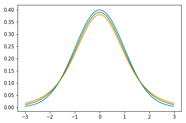
Note how the t-distributions have a bell shape like the normal, but have lower maximum and fatter tails.

Next, let’s plot a standard normal (blue) and a t with $\nu=100$ (green):

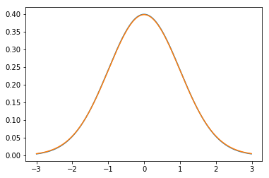
At a moderate sample size of $N=100$ there is effectively no difference between the distributions.

The t-test becomes the z-test at $ N = 100 $

As $ N \rightarrow \infty $:

• the t-distribution becomes a normal distribution
• the final outcome of hypothesis testing, the p-value becomes identical for a t-test and a z-test.

The difference effectively disappears at around $N=100$ sample size. So if you’re performing a timespent A/B test, and you have 100s or more samples in each bucket, the t-test and the z-test will yield numerically identical results. This is becauce at such sample sizes, the estimate of $s^2$ for $\sigma_p^2$ becomes really good for estimating the mean, and it’s divided by $N$ anyway, so the importance of the estimate goes down with increasing $N$.

When googling for “z test vs t test”, a lot of advice goes like “use the t-test if you don’t know the variance” and “use the t-test for $N<100$”. This is not incorrect, but it’s a bit confusing. For A/B testing, a clear and concise statement is: in A/B testing you never know the population mean, you’re estimating it, so always use the t-test. For $N>100$, the t-test numerically yields the same results as the z-test.

Simulating p-values

Let’s perform a Monte-Carlo simulation to see how the t-test becomes the z-test. The statsmodel package has both t and z-tests (1 sided and 2 sided). Let’s assume we have true populations for A and B, we take some samples from both to estimate the mean, and we perform both a t-test and a z-test to get 1-sided p-values. We then compute the average and maximum absolute p-value difference:

def simulate_p_values(population_A, population_B, sample_size_A, sample_size_B, num_simulations=100):
    p_diffs = []
    for _ in range(num_simulations):
        sample_A = population_A.rvs(size=sample_size_A)
        sample_B = population_B.rvs(size=sample_size_B)
        t_stat = ttest_ind(sample_A, sample_B, value=0, alternative='larger')
        z_stat = ztest(sample_A, sample_B, value=0, alternative='larger')
        p_diff = abs(z_stat[1] -  t_stat[1])
        p_diffs.append(p_diff)
    return mean(p_diffs), max(p_diffs)

Let’s see what happens if we assume that both A and B are identical exponentials (so the null hypothesis is true), and we very sample size from 10 to 500:

p_diffs = []
for sample_size in range(10, 500):
    p_diff = simulate_p_values(
        population_A=expon,
        population_B=expon,
        sample_size_A=sample_size,
        sample_size_B=sample_size
    )
    p_diffs.append(p_diff)
plt.xlabel('sample size')
plt.ylabel('|p z-test - p t-test|')
plt.plot(p_diffs)
plt.show()

The output is (blue is mean, orange is maximum absolute p-value difference across 100 A/B tests performed at each sample size):

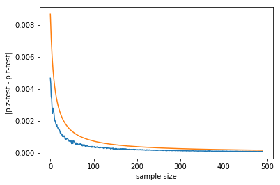
Note that:

• the difference tends to 0 with increasing sample size
• the p-value differences shown are on the order of 0.001, in real life we usually work with p-values between 0.01 and 0.05

Let’s see what happens when the A/B test is actually working, ie. B has better timespent on average (so the null hypothesis is false). To make the effect more visible, let’s pretend that timespent doubled. For this, we just have to change the lines:

    population_A=expon(loc=1),
    population_B=expon(loc=2),

in the above code. This yields:

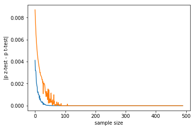
Comparing with the above (null hypothesis is true), in such a case the p-value difference drops even quicker. This makes sense: if there is an effect (null hypothesis is false), the tests return a lower p-value, so the difference will also be lower.

Conclusion

In a timespent A/B test scenario, we should always use the t-test. Both the t and z-tests are a library call, so there’s no difference in effort. For real-life high sample size use-cases, numerically there’s no difference in the p-values computed. However, the z-test is a much simpler mental model, as it models the test statistic as the intuitive normal distribution and there’s no degrees of freedom involved like in the t-distribution. So, my rule of thumb: use the t-test, pretend it’s a z-test.