A/B testing and the Z-test

Introduction

In the previous two posts, we talked about the A/B testing and the Central Limit Theorem and discussed when the CLT doesn’t hold in Beyond the Central Limit Theorem (CLT). The next step in exploring A/B testing is to look at the Z-test, which is the most common and straightforward staistical test.

With our understanding of the CLT, the Z-test is simple to explain. We’re running a Z-test if:

• our null hypothesis is the relationship between population means or other test statistics, and
• we can assume that the CLT holds and the test statistics follow a normal distribution

The same from Wikipedia:

A Z-test is any statistical test for which the distribution of the test statistic under the null hypothesis can be approximated by a normal distribution.

The code shown below is up on Github.

Statistical hypothesis testing

In a conversion A/B test setting, statistical hypothesis testing is:

• we have a base version A and contender version B, and we’re trying to decide whether B is better than A
• if B is converting worse than A, then we’re done
• if B is converting better than A, we’d like to know how significant our results are; in hypothesis testing, we compute the probability that we’d get this result if B is actually not better than A; ie. we compute the probability of getting the result that B is better than A due to random chance, even if B is not better than A; this probability is called the p-value

To get a better feeling for the point above, imagine if somebody gives you a coin. They claim it’s a fair coin, meaning you get Heads and Tails half the time. You want to test this claim, ie. the null hypothesis of a fair coin. If you flip it 10 times, and you get 6 Hs and 4 Ts, how confident are you that it’s not a fair coin? You can’t be too sure, because you haven’t collected enough samples, because the 6:4 result is a very likely outcome even if the coin is fair. The 6:4 result is not significant enough to disprove the null hypothesis of a fair coin. But if you flip it 1000 times, and you get 599 Hs and 401 Ts, that’s quite suspicious. Getting 599:401 from a fair coin is unlikely (it can be calculated explicitly, see below).

Types of Z-tests

Some points to make our thinking about the Z-test clear.

It’s called Z-test because when running the numbers, it’s common to transform the data to a standard normal distribution $N(0, 1)$. In the old days, before computers, the p-value, ie. the portion of the normal distribution outside the normalized test statistic (eg. the difference of the means) would be read off a printout table (eg. the back of statistics textbooks), and this statistic is conventionally denoted with the letter z. A more verbose, but descriptive name would be test-for-normally-distributed-test-statistics.

The Z-test is not one specific test, it’s a kind of test. Any time we work with an approximately normally distributed test statistic, we’re performing a Z-test. The practical bible of statistical testing, 100 Statistical Tests by Gopal Kanji, lists the following types of Z-tests:

• Test 1: Z-test for a population mean (variance known)
• Test 2: Z-test for two population means (variances known and equal)
• Test 3: Z-test for two population means (variances known and unequal)
• Test 4: Z-test for a proportion (binomial distribution)
• Test 5: Z-test for the equality of two proportions (binomial distribution)
• Test 6: Z-test for comparing two counts (Poisson distribution)
• Test 13: Z-test of a correlation coefficient
• Test 14: Z-test for two correlation coefficients
• Test 23: Z-test for correlated proportions
• Test 83: Z-test for the uncertainty of events
• Test 84: Z-test for comparing sequential contingencies across two groups using the ‘log odds ratio’

I listed out these to further the point that the Z-test is not just one test, it’s a type of test that makes sense in a variety of scenarios.

Formulas

The math is similar to the discussion in the CLT post. We’re sampling a distribution and computing a test statistic, and assuming that it follows a normal distribution $ N(\mu, \sigma^2) $. In an A/B test, we have two normal distributions, $ N(\mu_A, \sigma_A^2) $ and $ N(\mu_B, \sigma_B^2) $ with samples sizes $N_A$ and $N_B$, and the test statistic is $ N(\mu_A, \sigma_A^2) - N(\mu_B, \sigma_B^2) = N(\mu = \mu_B - \mu_A, \sigma^2 = \sigma_A^2 + \sigma_B^2) $ by the addition rule for normal distributions.

The test statistic then is $ Z = \frac{ \mu }{ \sigma } $, we use this to get the p-value for the experiment. This is simply the normalized distance from the mean of the distribution. With this normalized distance, we can use a table for a standard normal distribution table and read off the p-value. In the age of computers, we actually don’t have to do this final normalization step to get Z, we can just get the p-value from the original $ N(\mu, \sigma^2) $ distribution.

In an A/B test setting, $ \mu_A $ and $ \mu_B $ are known. The trick is, what are the standard deviations $ \sigma_A^2 $ and $ \sigma_B^2 $? We compute it from the sample standard devation $ s^2 $, like $ \sigma^2 = s^2/N $. The sample standard deviation is:

• for conversion, the population distribution is Bernoulli, so $ s^2 = \mu(1-\mu) $
• for timespent, you can compute the standard error from the data directly $ s^2 = \frac{1}{N} \sum{(\mu - x_i)^2} $, where $x_i$ are the invididual timespents per user, and $ \mu = \frac{1}{N} \sum{ x_i } $.

Sample size

Before running an A/B test, we have to decide 2 things:

• $ \alpha $, the False Positive Rate (FPR): if B is actually not better than A, by chance the measurement can still show B to be better. We can reduce this by collecting more samples. But we need to set an FPR that we are okay with with. Usually people set this to 0.05, but as I discuss this in the previous post A/B tests: Moving Fast vs Being Sure, startups should favor velocity over certainty, using 0.1 or 0.2 is fine.
• $ 1 - \beta $, the True Positive Rate (TPR) or power: if B is actually better than A, how likely are we to actually measure B to be better at the above $ \alpha $? If we don't account for this, by default the math will work out set $ \beta = 0.5 $, which means we will only find half of the good Bs. In real life we usually set power to 0.8. For more on power, see this article. We usually set power to 0.8.

Simulating an A/B test

Let’s pretend we’re running an A/B test on funnel conversion. A is the current, B is the new version of the funnel. We want to know whether B is better. By looking at our funnel dashboard, we know that A is historically converting around 9-11%.

Step 1. Formulate the action hypothesis: B has higher conversion than A, meaning we're doing a one-sided test.

Step 2. We set $ \alpha = 0.10 $ and $ 1 - \beta = 0.80 $. This means we're okay with 10% false positives and we will capture 80% of improvements.

Step 3. Decide traffic split. Let’s say we will keep 80% in A, 20% in B. This is how much of a chance we take, B could be worse, buggy, etc.

Step 4. Figure out how many samples we need to collect, given the historic conversion, traffic split, alpha and the kind of lift we’re looking. The code below computes sample size based on the math above:

from scipy.stats import norm

def alpha_to_z(alpha, one_sided):
    if one_sided:
        pos = 1 - alpha
    else:
        pos = 1 - alpha/2.0
    return norm.ppf(pos)

def power_to_z(power):
    pos = power
    return norm.ppf(pos)

def num_samples(alpha, mu_A, mu_delta, traffic_ratio_A, power=0.50, one_sided=True):
    z_alpha = alpha_to_z(alpha, one_sided)
    z_power  = power_to_z(power)
    mu_B = mu_A + mu_delta
    traffic_ratio_B = 1 - traffic_ratio_A
    N = ( mu_A*(1-mu_A)/traffic_ratio_A + mu_B*(1-mu_B)/traffic_ratio_B ) * ((z_alpha+z_power)**2) / (mu_A - mu_B)**2  
    return math.ceil(N)

Note that in real-life, there are other considerations. For example, if possible we should run tests for complete days and/or weeks, to capture users who are active at different times. So when we calculate the sample size, in real life we compare that to the number of users going through the funnel per day/week, and "round up". To take this into account in the simulation below, I will multiply by 2.

Step 5. Create a random seed for the A/B test and save it server-side. We generate a new seed for each A/B test. Let’s say we generate the string for this one: OkMdZa18pfr8m5sy2IL52pW9ol2EpLekgakJAIZFBbgZ

Step 6. Perform test by splitting users randomly between A and B according to the above proportions. Users coming, identified by a user_id (or cookie_id), should be put in the same funnel. We can accomplish this by hashing the test_id, where test_id = seed + user_id:

import hashlib

test_seed = 'OkMdZa18pfr8m5sy2IL52pW9ol2EpLekgakJAIZFBbgZ'

def funnel_user(base_traffic_split, test_seed, user_id):
    test_id = hashlib.md5(test_seed.encode('ascii') + str(user_id).encode('ascii')).hexdigest()
    bits = bin(int(test_id, 16))[3:]
    r = sum([int(bit)*(0.5**(i+1)) for i, bit in enumerate(bits)])
    if r < base_traffic_split:
        return 'A'
    else:
        return 'B'

Step 7. Run the test. We're simulating the real-world here, so we will have to pick the actual conversions for A and B. This is not known to the test, this is what it's trying to estimate, so we call this a hidden variable:

hidden_conversion_params = {'A': 0.105, 'B': 0.115 }

def run_test(N, hidden_conversion_params, funnel_user_func):
    test_outcomes = {'A': {'N': 0, 'conversions': 0}, 'B': {'N': 0, 'conversions': 0}}
    for user_id in range(N):
        which_funnel = funnel_user_func(user_id) # returns 'A' or 'B'
        test_outcomes[which_funnel]['N'] += 1
        if random() < hidden_conversion_params[which_funnel]:
            test_outcomes[which_funnel]['conversions'] += 1
    return test_outcomes

Step 8. Compute the p-value and compare it with the $ \alpha $ we set to decide whether to accept or reject B:

def p_value(N_A, mu_A, N_B, mu_B, one_sided=True):
    sigma_A_squared = mu_A * (1 - mu_A) / N_A
    sigma_B_squared = mu_B * (1 - mu_B) / N_B
    sigma_squared = sigma_A_squared + sigma_B_squared
    z = (mu_B - mu_A) / math.sqrt(sigma_squared)
    p = z_to_p(z, one_sided)
    return p

alpha = 0.10
power = 0.80
base_conversion = 0.10
valuable_diff = 0.01
base_traffic_split = 0.8

N_required = num_samples(
    alpha=alpha,
    mu_A=base_conversion,
    mu_delta=valuable_diff,
    traffic_ratio_A=base_traffic_split,
    power=power,
)
N_actual = 2 * N_required # because eg. we run it for a whole week

# hidden_conversion_params is how our funnels actually perform:
# the difference between the two is what we're trying to establish
# with statistical confidence, using an A/B test
hidden_conversion_params = {'A': 0.105, 'B': 0.115 }
test_seed = 'OkMdZa18pfr8m5sy2IL52pW9ol2EpLekgakJAIZFBbgZ'
test_outcomes = run_test(
    N_actual,
    hidden_conversion_params,
    lambda user_id: funnel_user(base_traffic_split, test_seed, user_id),
)

print(test_outcomes)

mu_A = test_outcomes['A']['conversions'] / test_outcomes['A']['N']
mu_B = test_outcomes['B']['conversions'] / test_outcomes['B']['N']

print('Measured conversion for A: %.3f' % mu_A)
print('Measured conversion for B: %.3f' % mu_B)
p = p_value(test_outcomes['A']['N'], mu_A, test_outcomes['B']['N'], mu_B)
print('p-value: %.3f' % p)
if p <= alpha:
    print("""B is better, deploy""")
else:
    print("""We're not sure if B is better than A""")

The outcome depends on chance, here's one run:

{'A': {'N': 43464, 'conversions': 4620}, 'B': {'N': 10812, 'conversions': 1222}}
Measured conversion for A: 0.106
Measured conversion for B: 0.113
p-value: 0.023
Action: B is better, deploy

If you run this repeatedly, sometimes it will indicate B is better, sometimes it will not. It will find B better more often:

• at higher $ N $, if in fact B is better
• if the conversion advantage of B is greater in the hidden conversion parameters

Consistency test for FPR ($\alpha$)

We can set the A and B equal in the hidden conversion parameters, repeatedly perform the A/B test, and count the ratio of times it finds B to be better than A at the $ \alpha $ level, ie. the ratio of false positives. It should be equal to the $ \alpha $ we set to compute the sample size!

num_tests = 1000
alpha = 0.10
base_conversion = 0.10
valuable_diff = 0.01
base_traffic_split = 0.8
hidden_conversion_params = {'A': 0.10, 'B': 0.10 }
N = num_samples(
    alpha=alpha,
    mu_A=base_conversion,
    mu_delta=valuable_diff,
    traffic_ratio_A=base_traffic_split,
)

# get rid of this of the hashing, it's slow, we don't need it for a simulation
def funnel_user(base_traffic_split):
    if random() < base_traffic_split:
        return 'A'
    else:
        return 'B'

def run_tests(num_tests, N, alpha, hidden_conversion_params, funnel_user_func):
    num_successes = 0
    for i in range(num_tests):
        test_outcomes = run_test(
            N,
            hidden_conversion_params,
            funnel_user_func,
        )
        mu_A = test_outcomes['A']['conversions'] / test_outcomes['A']['N']
        mu_B = test_outcomes['B']['conversions'] / test_outcomes['B']['N']
        p = p_value(test_outcomes['A']['N'], mu_A, test_outcomes['B']['N'], mu_B)
        if p <= alpha:
            num_successes += 1
    return num_successes

num_successes = run_tests(
    num_tests,
    N,
    alpha,
    hidden_conversion_params,
    lambda _: funnel_user(base_traffic_split),
)

fpr = num_successes/num_tests
print("False Positive Rate = %.2f (expected = %.2f)" % (fpr, alpha))

It prints:

False Positive Rate = 0.10 (expected = 0.10)

Consistency test for TPR ($1 - \beta$)

We can set the A and B hidden conversion parameters exactly like the assumption we used to compute the sample size (ie. 10% and 11%), repeatedly perform the A/B test, and count the ratio of times it finds B to be better than A at the $ \alpha $ level. It should be equal to the $ 1 - \beta $ power we set to compute the sample size!

num_tests = 1000
alpha = 0.10
power = 0.80
base_conversion = 0.10
valuable_diff = 0.01
base_traffic_split = 0.8
hidden_conversion_params = {'A': 0.10, 'B': 0.11 }
N = num_samples(
    alpha=alpha,
    power=power,
    mu_A=base_conversion,
    mu_delta=valuable_diff,
    traffic_ratio_A=base_traffic_split,
)

num_successes = run_tests(
    num_tests,
    N,
    alpha,
    hidden_conversion_params,
    lambda _: funnel_user(base_traffic_split),
)

tpr = num_successes/num_tests
print("True Positive Rate: %.2f (expected = %.2f)" % (tpr, power))

It prints:

True Positive Rate: 0.80 (expected = 0.80)

Scaling behaviour

Let's fix all parameters but one, and see how many samples we need.

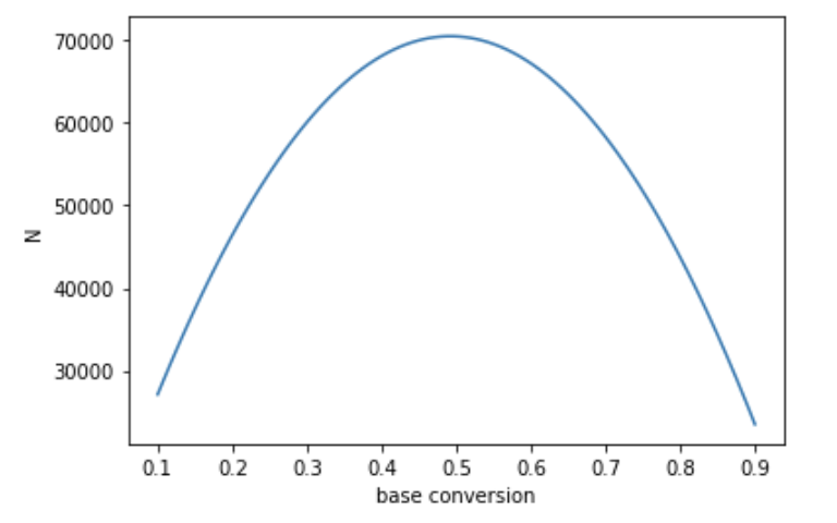
Vary base conversion $\mu_A$, with fixed $ \mu_B - \mu_A, \alpha, 1 - \beta$, traffic split. Because the formula for $z$ includes a term like $\mu_A(1-\mu_A)$, this should be highest at $\mu_A=0.5$.

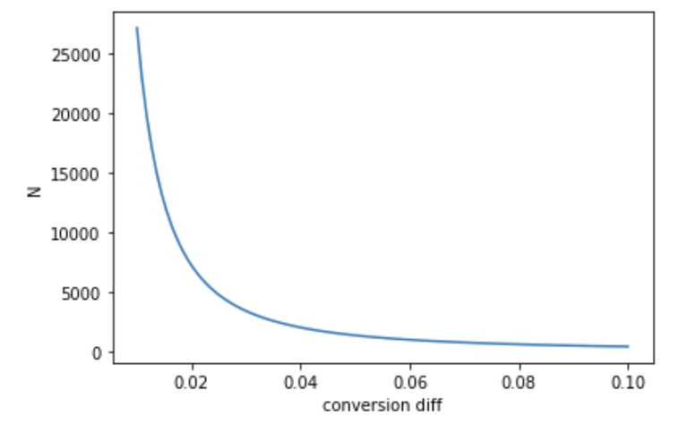
Vary conversion difference $\mu_B - \mu_A$, with fixed $ \mu_A, \alpha, 1 - \beta$, traffic split. A higher conversion difference requires less samples to detect.

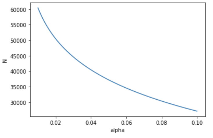
Vary $\alpha$, with fixed $ \mu_A, \mu_B - \mu_A, 1 - \beta$, traffic split. Lower $\alpha$ means we want less false positives, which requires more samples.

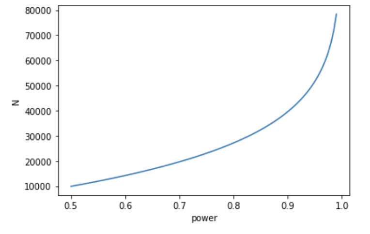
Vary the power $1 - \beta$, with fixed $ \mu_A, \mu_B - \mu_A, \alpha$, traffic split. Higher $1 - \beta$ translates to higher probability of detecting positive outcomes, which requires more samples.

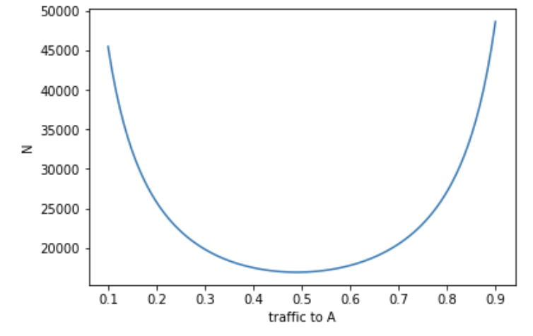
Vary the traffic split to A, with fixed $ \mu_A, \mu_B - \mu_A, \alpha, 1 - \beta$. The sample size is constrained by the smaller sample size of the two, so an equal split requires the least amount of samples.

Conclusion

Z-tests are simple, if you remember the CLT and are careful about controlling false positive rate and true negatives rates. If in doubt, write simulation code like above and make sure the way you set your parameters gets you the results you want. Also remember that there are other types of tests, such as the $\chi^2$-test and the t-test, to be discussed in the next posts.

Related links:

• The Art of A/B Testing - good post on the same topic