Calibration curves for delivery prediction with Scikit-Learn

Introduction

In a previous post about Machine Learning at Fetchr, I mentioned several families of models we have in production. The latest is Operational Choice, which we use for delivery prediction. The idea is simple: we have a large number of features (essentially columns in our data warehouse) available for our historic dispatches:

• sender's information
• recipient’s information (address, etc.)
• recipient’s historic information
• geography
• scheduling channel
• timing
• etc.

For each dispatch, we know whether it was successfully delivered or not (True/False). Given our historic data, we can build a binary classifier which predicts which orders will be delivered (or not) tomorrow, of all orders scheduled for dispatch. After one-hot encoding, our feature vector length is in the 1000s, and we can achieve 90%+ accuracy with out-of-the-box Scikit-Learn models. In other words, perhaps not too surprisingly, it is possible to predict the chances of delivery success quite well.

When using this in production, we don’t primarily look at the absolute value of the delivery probability itself. What we care about is the relative ordering: out of 1,000 orders, which are the least likely to be delivered successfully tomorrow? Operational Choice is about treating these orders differently. So while in standard ML classification tasks usually the most important metric is accuracy (assuming a balanced dataset), ie. the ratio of test data that is predicted correctly by the predictor, here we also care about calibration: that the relationship between predicted and actual delivery probability should be monotonic, and as close to the x=y line as possible.

As a reminder, the way the binary (delivered or not) predictor models discussed here work is that given a feature vector, they return a probability of delivery, like 0.67 (SKL’s model.predict_proba() functions. If we want to get a True/False prediction, we cut the probability at 0.5, so for 0.67 we would predict True (SKK’s model.predict() function). Accuracy is the ratio of test data (historic dispatches) where the True/False prediction matches the actual True/False historic delivery outcome. To get the calibration curve, we need to convert the True/False historic ground truth to probabilities, so we need to bucket the data and count the ratio of successful deliveries.

Below I show the calibration results for 4 Scikit-Learn models:

• LogisticRegression
• DecisionTree
• RandomForest
• GradientBoosting

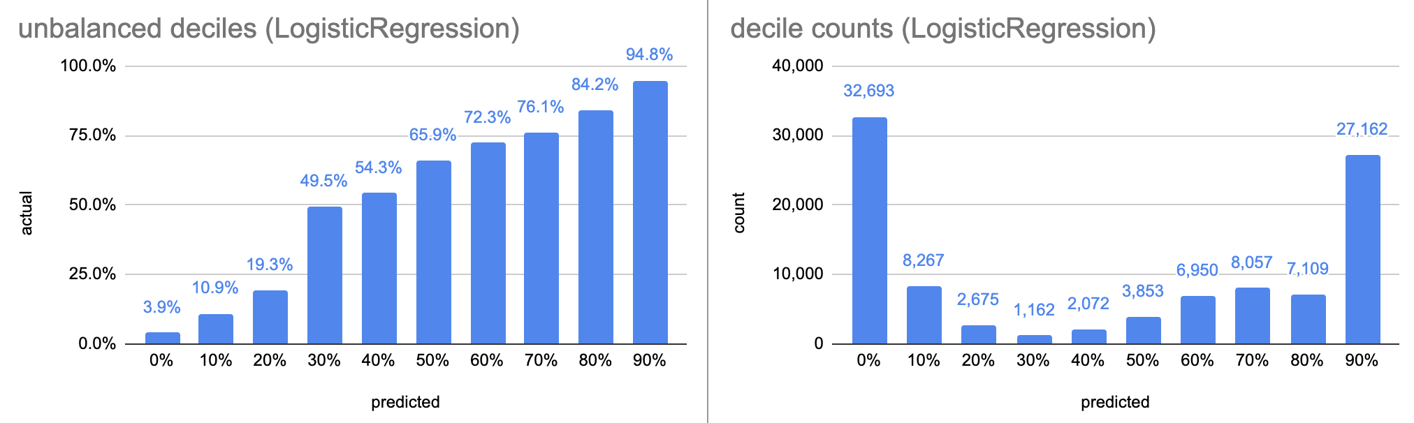
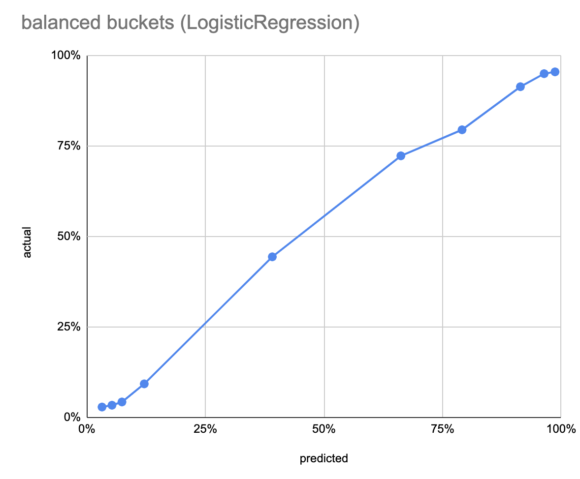
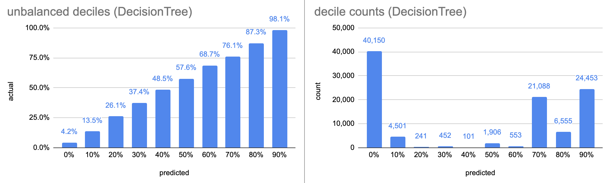
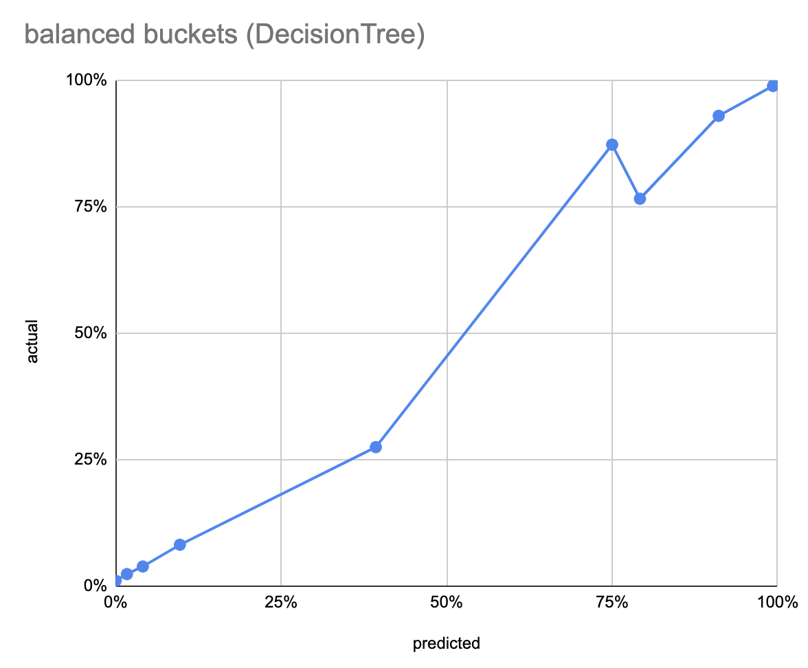
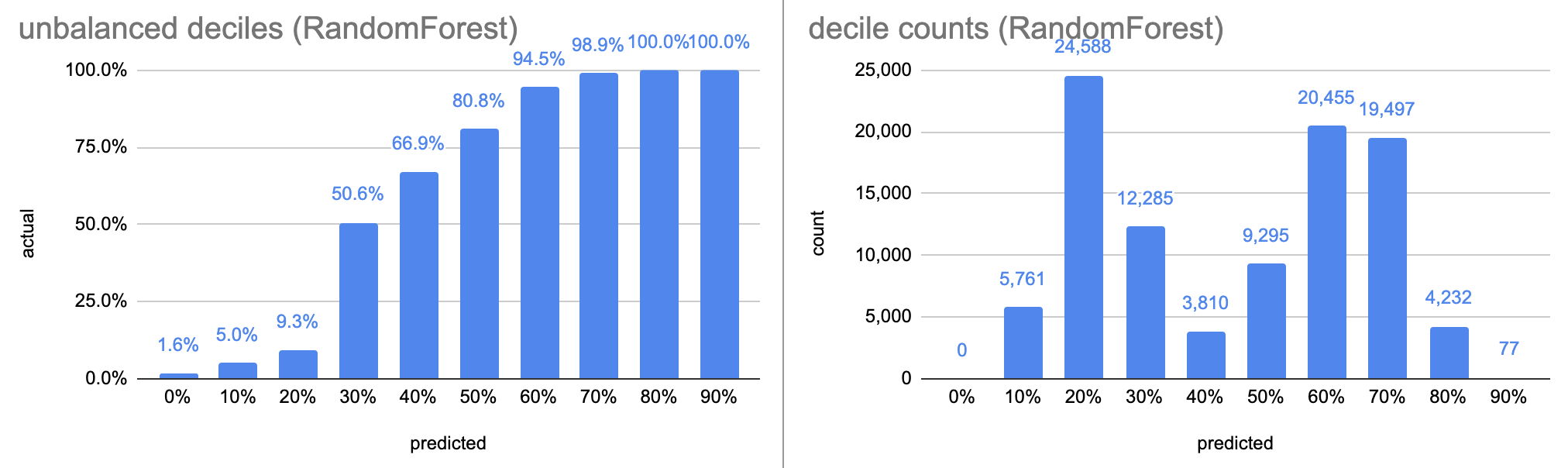
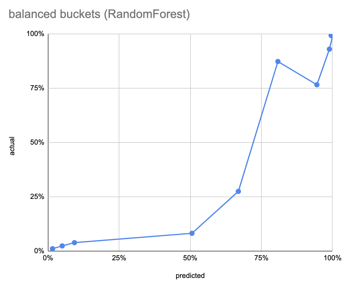
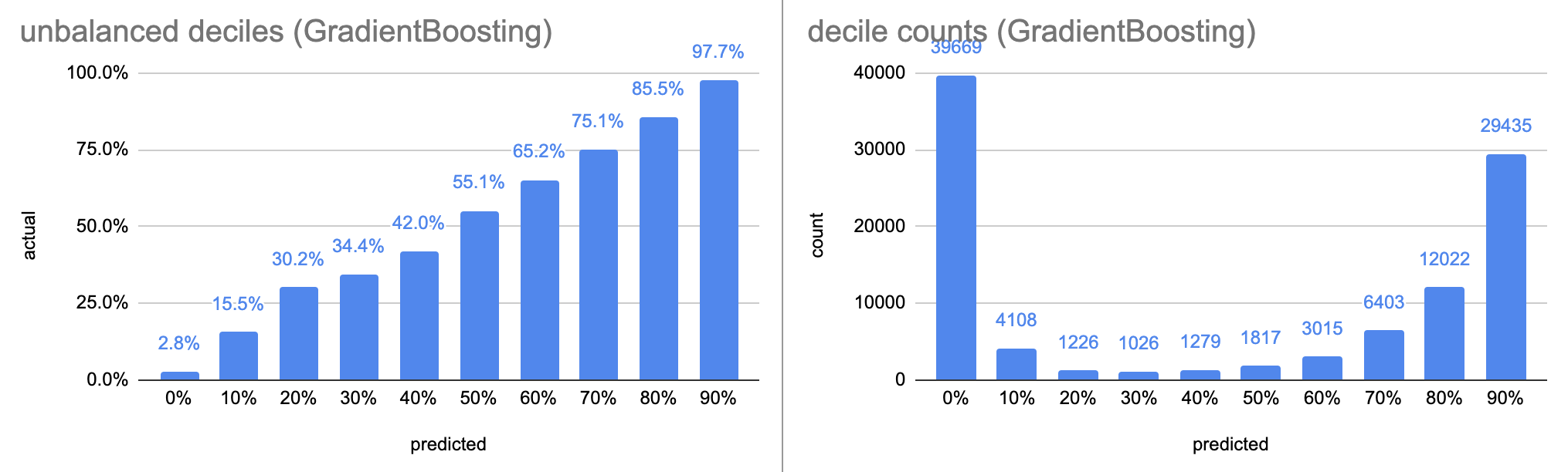
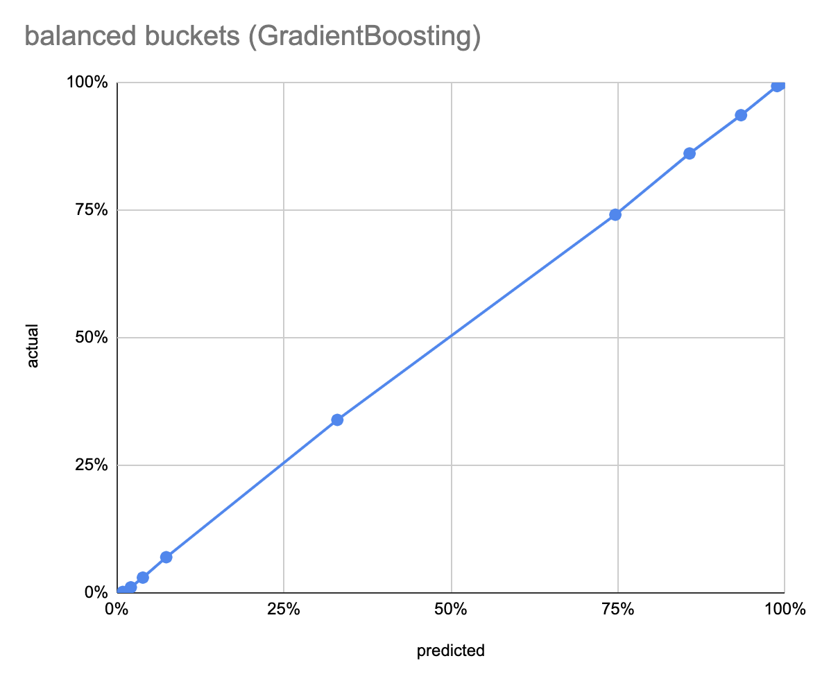
The first left chart show the predicted probability on the x-axis, by deciles, as a bar chart; so the first bar is test data points where the model predicted between 0-10% delivery probability, and so on. The y axis is the ratio of test data in the bucket that was actually delivered (ratio of Trues). The right chart shows the number of data points in each decile; since the deciles are fixed, the counts are unbalanced, which leads to inbalanced statistics, ie. the error varies between bars. The lower, third chart shows the same thing, but with equal bucket sizes (total 10 buckets).

To get these results, I used 100,000 randomly chosen training points from our real delivery data and 100,00 test points. Both sets were randomly chosen, so the test distribution matches the training distribution. Both are balanced 50-50 between successful and unsuccessful deliveries.

LogisticRegression

LogisticRegression is the simplest model, it takes 4 seconds to train. It has an accuracy of 87.9% on the balanced dataset. Both the unbalanced and balanced calibration curves look very good.

DecisionTree(max_depth=10)

The DecisionTree model, after 13 seconds of training, has an accuracy of 90.1%. The decile calibration curve is beautiful, although the deciles are very unbalanced, so this could be misleading. The balanced calibration curve has an inversion between the 7th and 8th buckets.

RandomForest(max_depth=10)

The RandomForest model, after 7 seconds of training, has an accuracy of 87.5%. The decile calibration curve is more like a sigmoid, and it’s interesting that the decile counts are skewed torwards the middle. The balanced calibration curve has an inversion between the 7th and 8th buckets, like the DecisionTree.

GradientBoosting(max_depth=10)

The GradientBoosting model, after 1,679 seconds of training (!), has an accuracy of 91.1%. Both the balanced and unbalanced calibration curves are very close to the ideal x=y. The decile counts are heavily skewed towards the two ends.

Discussion

If training time is not an issue, the GradientBoosting model is the best choice, both in terms of accuracy and in terms of calibration. Note how the subsequent gradient boosting steps push the predicted probabilities towards 0 and 1, resulting in the highly skewed decile counts. As a reminder, this is an ensemble of trees, trained and applied in sequence, where each subsequent tree is attempting to correct mistakes made so far; it's this construction which results in the skewed distribution.

It’s also interesting to see how well the LogisticRegression model performs. It’s (i) only 3% off in terms of accuracy from GradientBoosting (ii) in terms of calibration it’s very close to GradientBoosting (iii) it takes only 4 seconds to train, 400x faster than GradientBoosting.

The DecisionTree and the RandomForest models are not very appealing for this use-case. Note how the averaging between the trees in the RandomForest ensemble pulls the predicted probabilities towards 0.5. As a reminder, a DecisionTree cuts along a feature dimension at each step; when predicting, it travels down to a leaf, and returns the ratio of True training points in the leaf bucket. A RandomForest is an ensemble of such trees, with the final prediction being the average of the ensemble trees’ predictions.

Accuracy is usually the primary indicator of how good a classification model is performing. However, in thise case our primary goal is to extract the probabilities, so we can use them for Operational Choice, ie. ranking orders. An imaginary perfect predictor would return p=0 and p=1 at 100% accuracy (so ROC AUC=1). This would be valuable because then we could not dispatch the p=0 orders, since we could be 100% sure they wouldn't be delivered—but this is unrealistic. We actually prefer a model which nicely "stretches" the orders by the actual probability of delivery with a monotonic calibration curve, following the x=y diagonal, like the GradientBoosting model.