Comparing conversion at control and treatment sites

Introduction

In real-life, non-digital situations, it's often not feasible to run true A/B tests. In such cases, we can compare before and after rollout conversions at a treatment site, while using a similar control site to measure and correct for seasonality. The post discusses how to compute increasingly correct p-values and bayesian probabilities in such scenarios.

Imagine a cinema selling movie tickets and upselling food and beverages, and experimenting with different pricing to see how it affects upsell conversion. For simplicity, let's say non-conversion means a customer buys just a movie ticket, whereas a conversion means a customer buys a movie ticket plus some food and beverages. Since the cinema is a real-life venue (not digital) the pricing is shown on large printed banners, and can't be varied per arriving customer (there may also be legal reasons).

In such situations, the experiment setup is:

1. Treatment site: roll out the experimental pricing at the treatment site (let's day on Dec-1) and measure the change in conversion before vs. after rollout (let's say for a week).
2. Control site: don't make any changes, and measure the change in conversion before vs. after rollout. The control lift can be used to estimate and subtract out the "seasonal" change from the treatment effect.

It's important to note that even when using a control site, we're doing a best-effort estimation of conversion lift. We cannot be sure that any signal we pick up is due to the treatment we applied, and not some external factor. Some issues we face:

1. The populations of the before and after (and even the control and treatment site) are not distinct: a customer could show up both at the control and the treatment site, both before and after the rollout. This could result in unexpected spill-over effects. If possible, it's best to exclude such customers from the study.
2. The treatment site and the control site will never be statistically exactly the same, so any seasonal correction we measure at the control site is only an approximation of the treatment site's. For example, if a new Bollywood movie comes out after the treatment is applied at the treatment site, and one of the sites draws more people from India, who are more likely to buy food and beverages along with the movie ticket, that will skew the results.
3. It's possible that an external event, unrelated to the pricing change, is causing a change at one of the sites after the rollout, and the lift we're measuring is due to this external reason and not the pricing change. For example, there is a big shop next to one of the sites, which closes down during the treatment period and skews the mix of people coming in to this site site.

It would be tempting to say that "because of the above", only a strong signal (high lift, low p-value, high bayesian probability) should be accepted. But this is misleading, because external events like the above can cause a strong signal. The result of such a control vs treatment site analysis should only be accepted after careful checks of populations mixes along various splits, checking various metrics and other external factors (eg. nearby physical events) of the sites indicate that it's safe to proceed with the analysis.

Having laid out these caveats, the two main questions are:

1. How can we compute an estimated treatment lift?
2. How can we compute an estimated significance (or bayesian probability of "after" being better than "before")?

The code is up on Github.

Experiment setup

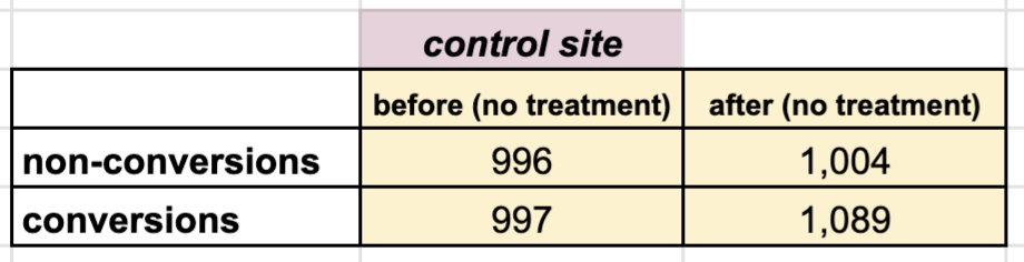
Let's use the following toy numbers. Our measurements at the control site, before and after the rollout date:

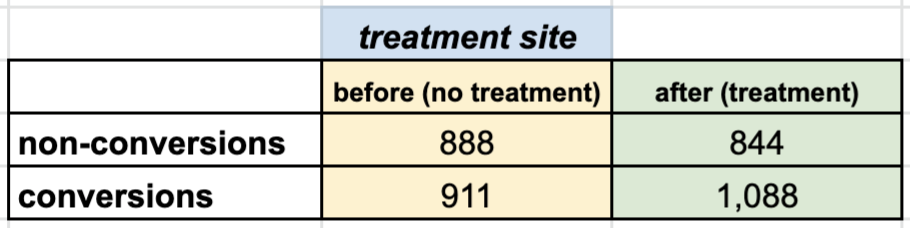
At the treatment site, where we actually change the price:

Estimating the treatment lift

At the control site, before rollout, conversion was $ 997 / (996+997) = 50 \% $, after rollout $ 1089 / (1004+1089) = 52 \% $, so the control's relative lift in conversion is $ 0.52 / 0.50 - 1 = 4 \% $. Since we didn't make any change at the control site, we assume that this lift is a seasonal lift. Doing the same at the treatment site, the uncorrected, raw relative lift is $ 11.2 \% $. Subtracting out the seasonal lift leaves us with $ 11.2 \% - 4 \% = 7.2 \% $ "real", corrected lift.

Let's code it up:

control_site = [
    [996, 1004],
    [997, 1089],
]

treatment_site = [
    [888,  844],
    [911, 1088],
]

conv_control_before = control_site[1][0] / (control_site[0][0] + control_site[1][0])
conv_control_after  = control_site[1][1] / (control_site[0][1] + control_site[1][1])
conv_control_lift = conv_control_after / conv_control_before - 1.0
print('conversion at control site before = %.2f' % conv_control_before)
print('conversion at control site after  = %.2f' % conv_control_after)
print('relative conversion lift at control = %.3f (assumed to be seasonality)' % conv_control_lift)
print()

conv_treatment_before = treatment_site[1][0] / (treatment_site[0][0] + treatment_site[1][0])
conv_treatment_after  = treatment_site[1][1] / (treatment_site[0][1] + treatment_site[1][1])
conv_treatment_lift = conv_treatment_after / conv_treatment_before - 1.0
conv_treatment_lift_corr = conv_treatment_lift - conv_control_lift
print('conversion at treatment site before = %.2f' % conv_treatment_before)
print('conversion at treatment site after  = %.2f' % conv_treatment_after)
print('relative conversion lift at treatment = %.3f (including assumed seasonality)' % conv_treatment_lift)
print()

print('relative conversion lift at treatment with correction (seasonality subtracted out) = %.3f' % conv_treatment_lift_corr)

Prints:

conversion at control site before = 0.50
conversion at control site after  = 0.52
relative conversion lift at control = 0.040 (assumed to be seasonality)

conversion at treatment site before = 0.51
conversion at treatment site after  = 0.56
relative conversion lift at treatment = 0.112 (including assumed seasonality)

relative conversion lift at treatment with correction (seasonality subtracted out) = 0.072

Approach 1: Naive estimate of the statistical significance of the treatment lift (wrong)

Based on the above analysis, it seems that the treatment worked, and taking into account seasonality, there is still a positive lift. But is it statistically significant? Naively, we could take the treatment site's contingency matrix, and compute a p-value from that:

print('p-value of original treatment site contingency matrix = %.3f' % chi2_contingency(treatment_site)[1])

Prints:

p-value of original treatment site contingency matrix = 0.001

But this is definitely not right, because we didn't take into account the fact that we normalized our conversion lift using the control site.

Approach 2: Estimate of the statistical significance using a corrected contingency matrix (flawed)

A less wrong approach is to re-normalize the treatment site's contingency matrix, and calculate a p-value from that. First, re-normalize, fixing the "after" sample size, and re-distributing the non-conversion and conversion counts according to the corrected "after" conversion (which excludes the seasonality we compute using the control):

def correct_treatment_contingency_matrix(treatment_site, conv_control_lift):
    conv_treatment_before = treatment_site[1][0] / (treatment_site[0][0] + treatment_site[1][0])
    conv_treatment_after  = treatment_site[1][1] / (treatment_site[0][1] + treatment_site[1][1])
    conv_treatment_lift = conv_treatment_after / conv_treatment_before - 1.0
    conv_treatment_lift_corr = conv_treatment_lift - conv_control_lift
    conv_treatment_after_corr = conv_treatment_before * (1 + conv_treatment_lift_corr)
    treatment_site_corr = deepcopy(treatment_site)
    N = treatment_site_corr[0][1] + treatment_site_corr[1][1]
    treatment_site_corr[0][1] = round((1 - conv_treatment_after_corr) * N)
    treatment_site_corr[1][1] = N - treatment_site_corr[0][1]
    return treatment_site_corr

treatment_site_corr = correct_treatment_contingency_matrix(treatment_site, conv_control_lift)

print('Original treatment site contingency matrix:')
print(np.array(treatment_site))
print('Corrected treatment site contingency matrix:')
print(np.array(treatment_site_corr))

Prints:

Original treatment site contingency matrix:
[[ 888  844]
 [ 911 1088]]
Corrected treatment site contingency matrix:
[[ 888  883]
 [ 911 1049]]

And now we can calculate a more meaningful p-value:

print('p-value of corrected treatment site contingency matrix = %.3f' % chi2_contingency(treatment_site_corr)[1])

Prints:

p-value of corrected treatment site contingency matrix = 0.029

Because the seasonality was positive, it corrected the positive lift to be lower, which naturally results in a higher p-value, less statistical significance.

Similar to the above, we can also use the corrected contingency matrix to calculate the Bayesian probability that the conversion at the treatment site is higher after the treatment was applied vs before. I've described in detail how to calculate Bayesian conversion probabilities in this previous post. We can either use a closed form solution or use Monte Carlo sampling to compute the probability. Since we will use Monte Carlo simulations later anyway, let's go that route:

def sample_conversion_lifts(site_contingency, num_samples = 10*1000):
    beta_before = beta(site_contingency[1][0], site_contingency[0][0])
    beta_after  = beta(site_contingency[1][1], site_contingency[0][1])
    samples_before = beta_before.rvs(size=num_samples)
    samples_after  = beta_after.rvs(size=num_samples)
    return samples_before, samples_after

def bayesian_prob_after_gt_before(site_contingency, num_samples = 10*1000):
    samples_before, samples_after = sample_conversion_lifts(site_contingency, num_samples)
    hits = sum([after > before for before, after in zip(samples_before, samples_after)])
    return hits/num_samples

print('P(conv_after > conv_before | treatment_site     ): %.4f' % bayesian_prob_after_gt_before(treatment_site))
print('P(conv_after > conv_before | treatment_site_corr): %.4f' % bayesian_prob_after_gt_before(treatment_site_corr))

Prints:

P(conv_after > conv_before | treatment_site     ) = 0.9997
P(conv_after > conv_before | treatment_site_corr) = 0.9859

The story is the same as above: since the corrected conversion lift is lower, the probability of the effect being real is a bit lower ($ 98.6 \% $ vs $ 99.9 \% $).

Approach 3: Using Bayesian Monte Carlo methods to take into account the sample size at the control site (still flawed)

From a mathematical perspective, the big shortcoming of the above analysis (both the frequentist p-value and the bayesian) is that it ignores the sample size at the control site. In other words, when we compute conv_control_lift and then conv_treatment_lift_corr:

conv_control_lift = conv_control_after / conv_control_before - 1.0
...
conv_treatment_lift_corr = conv_treatment_lift - conv_control_lift

We take the conv_control_lift point estimate at face value, without taking into account that this lift at the control site is also a random variable, with spread around a mean. It could also be just random fluctuation.

To model the uncertainty at the control site, we can use the Beta distribution we know from Bayesian A/B testing and perform a Monte Carlo simulation.

1. Model the "before" conversion at the control site with a Beta distribution.
2. Model the "after" conversion at the control site with a Beta distribution.
3. In a Monte Carlo simulation, num_samples times:
4. Draw pairs of "before" and "after" conversion probabilities from the above distributions, and using these sampled conversions compute a sampled control conversion lift.
5. Using the sampled conversion lift, repeat the frequentist or bayesian analysis above to get a p-value or a bayesian probability

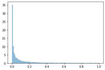
First, code and visualization for steps:

num_samples = 100*1000
samples_conv_control_before, samples_conv_control_after = sample_conversion_lifts(control_site, num_samples)
samples_conv_control_lift = [after/before-1 for before, after in zip(samples_conv_control_before, samples_conv_control_after)]
plt.hist(samples_conv_control_lift, bins=100, density=True, alpha=0.5)
plt.show()
print('mean relative conversion lift at control = %.3f (assumed to be seasonality)' % np.mean(samples_conv_control_lift))

Prints:

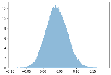
mean relative conversion lift at control = 0.041 (assumed to be seasonality)

We can then feed these sampled lifts at the control site into our subsequent calculations. Code for the frequentist p-value case:

def p_value_corr(treatment_site, conv_control_lift):
    treatment_site_corr = correct_treatment_contingency_matrix(treatment_site, conv_control_lift)
    return chi2_contingency(treatment_site_corr)[1]

num_samples = 100*1000
samples_conv_control_before, samples_conv_control_after = sample_conversion_lifts(control_site, num_samples)
samples_conv_control_lift = [after/before-1 for before, after in zip(samples_conv_control_before, samples_conv_control_after)]
ps = [p_value_corr(treatment_site, lift) for lift in samples_conv_control_lift]
plt.hist(ps, bins=100, density=True, alpha=0.5)
plt.show()
print('p-value of corrected treatment site contingency matrix (taking into account control site uncertainty) = %.3f' % np.mean(ps))

Prints:

p-value of corrected treatment site contingency matrix (taking into account control site uncertainty) = 0.115

Note that this is a significant adjustment: without taking into account the control site's uncertainty, the p-value was 0.029, but if we take it into account, it's 0.115, or 4x.

We can repeat the same to get an adjusted Bayesian probability:

def bayesian_prob_corr(treatment_site, conv_control_lift):
    treatment_site_corr = correct_treatment_contingency_matrix(treatment_site, conv_control_lift)
    return bayesian_prob_after_gt_before(treatment_site_corr)

num_samples = 10*1000
samples_conv_control_before, samples_conv_control_after = sample_conversion_lifts(control_site, num_samples)
samples_conv_control_lift = [after/before-1 for before, after in zip(samples_conv_control_before, samples_conv_control_after)]
bs = [bayesian_prob_corr(treatment_site, lift) for lift in samples_conv_control_lift]
plt.hist(bs, bins=100, density=True, alpha=0.5)
plt.show()
print('P(conv_after > conv_before | treatment_site_corr) (taking into account control site uncertainty) = %.3f' % np.mean(bs))

Prints:

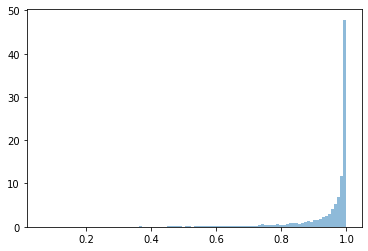
P(conv_after > conv_before | treatment_site_corr) (taking into account control site uncertainty) = 0.942

Similar to the frequentist case, this is a significant adjustment: without taking into account the control site's uncertainty, the probability was $ 98.5 \% $, while this calculation yields a more realistic $ 94.2 \% $. Like in the frequentist case, $ 1-P $ increases by 4x.

Approach 4: Pure Bayesian Monte Carlo approach without contingency matrix correction (best)

The problem with Approach 2 and 3 is that correcting the treatment site's contingency matrix is not statistically sound. It's like computing probabilities of a pretend measurement.

Fortunately, we can compute correct probabilities directly in a pure bayesian approach with Monte Carlo sampling. The approach is:

1. Model the "before" conversion at the control site with a Beta distribution.
2. Model the "after" conversion at the control site with a Beta distribution.
3. Model the "before" conversion at the treatment site with a Beta distribution.
4. Model the "after" conversion at the treatment site with a Beta distribution.
5. Sample the above distributions, and directly compute the control lift, treatment lift, and the corrected treatment lift.
6. Calculate the ratio of samples where the corrected treatment lift > 0.

Code:

def sample_conversion_lifts(site_contingency, num_samples = 100*1000):
    beta_before = beta(site_contingency[1][0], site_contingency[0][0])
    beta_after  = beta(site_contingency[1][1], site_contingency[0][1])
    samples_before = beta_before.rvs(size=num_samples)
    samples_after  = beta_after.rvs(size=num_samples)
    return samples_before, samples_after

samples_control_before, samples_control_after = sample_conversion_lifts(control_site)
samples_treatment_before, samples_treatment_after = sample_conversion_lifts(treatment_site)

def calculate_conv_treatment_lift_corr(conv_control_before, conv_control_after, conv_treatment_before, conv_treatment_after):
    conv_control_lift = conv_control_after / conv_control_before - 1.0
    conv_treatment_lift = conv_treatment_after / conv_treatment_before - 1.0
    conv_treatment_lift_corr = conv_treatment_lift - conv_control_lift
    return conv_treatment_lift_corr

lift_corrs = [calculate_conv_treatment_lift_corr(conv_control_before, conv_control_after, conv_treatment_before, conv_treatment_after)
     for conv_control_before, conv_control_after, conv_treatment_before, conv_treatment_after
         in zip(samples_control_before, samples_control_after, samples_treatment_before, samples_treatment_after)]

plt.hist(lift_corrs, bins=100, density=True, alpha=0.5)
plt.show()

p = sum([lift_corr > 0 for lift_corr in lift_corrs])/len(lift_corrs)

print('MC mean relative conversion lift at treatment with correction (seasonality subtracted out) = %.3f' % np.mean(lift_corrs))
print('P(corrected conversion lift > 0 at treatment site | control_site, treatment_site) = %.3f' % p)

Prints:

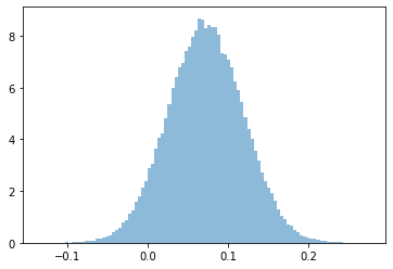
MC mean relative conversion lift at treatment with correction (seasonality subtracted out) = 0.072
P(corrected conversion lift > 0 at treatment site | control_site, treatment_site) = 0.938

Note that here the mean relative conversion lift of the Monte Carlo simulation ($ 7.2 \%) matches the point estimate from the beginning.

Why the control site's sample size matters

It's easy to see why by dividing the control site's contingency matrix by 10. Note that the point estimate of the corrected lift does not change, it's still $ 7.2 \% $, since it's just a function of ratios. Let's see what happen if we re-run the above code (approach 4), which is sensitive to sample size:

control_site = [
    [99.6, 100.4],
    [99.7, 108.9],
]
# same as above

A smaller sample size means our estimate of the seasonality is less accurate, so we expect to be less certain about our treatment lift:

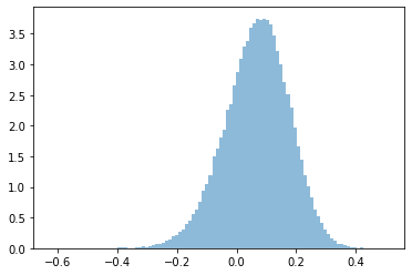
MC mean relative conversion lift at treatment with correction (seasonality subtracted out) = 0.067
P(corrected conversion lift > 0 at treatment site | control_site, treatment_site) = 0.745

In the Bayesian Monte Carlo method, at this low control sample size, since the spread is not symmetric about the mean, the mean relative lift actually goes down from $ 7.2 \% $ to $ 6.7 \% $, and our certainty that this effect is real goes down from $ 93.8 \% $ to $ 74.5 \% $!

Conclusion

The main takeaways here are:

1. When conducting such treatment vs control site experiments, we must conduct extensive internal checks to minimize the risk of external effects polluting our measurement.
2. We have to take into account the uncertainty of the control site. The cleanest approach is the pure bayesian Monte Carlo method.