Bayesian A/B conversion tests

Introduction

The A/B tests I talked about before, such as the Z-test, t-test, $\chi^2$ test, G-test and Fisher’s exact test are so-called frequentist hypothesis testing methodologies. In frequentist inference, we formulate a $H_0$ null hypothesis and an $H_1$ action hypothesis, run the experiment, and then calculate the $p_f$ value ($f$ for frequentist), which is the probability of the outcome of the experiment being at least as extreme as the actual outcome, assuming the null hypothesis $H_0$ is true. For one-tailed conversion tests, $H_0$ is “B is converting worse or the same as A” and $H_1$ is “B is converting better than A”. In the frequentist setting, if the $p_f$ value is lower than some threshold $\alpha$ (usually $\alpha=0.01$ or $\alpha=0.05$), then we reject the null hypothesis, and accept the action hypothesis.

At a high level, bayesian inference turns this on its head and computes the probability $p_b$ ($b$ for bayesian) that $H_1$ is true (and $H_0$ is false) given the outcome of the experiment. If this probability is high, we accept the action hypothesis.

Bayesian inference is a method of statistical inference in which Bayes' theorem is used to update the probability for a hypothesis as more evidence or information becomes available.

We expect that the two are related: if there is a big difference in conversion in favor of B versus A, relative to the sample size $N$, we expect to get a low frequentist $p_f$ value and a high $p_b$ bayesian probability. However, in terms of the math, the two are not complementary probabilities: $p_f + p_b \neq 1$. However, as I will show here, this relationship approximately holds when doing conversion 2x2 A/B testing with Beta distributions and flat priors: $p_f + p_b \simeq 1 $.

The code shown below is up on Github.

Conversion parameter estimation with the Beta distribution

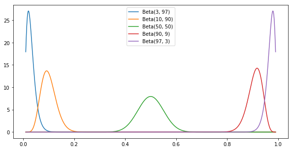
In Bayesian modeling, we pick a distribution to model the $\mu$ conversion probability for each funnel A and B. In other words, we say “I don’t know what the conversion of A is, but based on the experimental outcome, $P_A(\mu)$ is the probability that it is $\mu$.” For conversion modeling, we usually pick the Beta distribution to model the $\mu$ conversion parameter. The Beta distribution has two parameters, $\alpha$ and $\beta$, its peak is at $\frac { \alpha }{ \alpha + \beta }$, its domain is the range $[0, 1]$. Given an experimental outcome where we observed $C$ conversions out of $N$ cases, we set $\alpha=C$ and $\beta=N-C$, so $\alpha$ is the conversion count, $\beta$ is the non-conversion count. The Beta distribution is available in scipy, it’s easy to visualize:

N = 100
convs = [0.03, 0.10, 0.50, 0.90, 0.97]
plt.figure(figsize=(10,5))
x = np.linspace(0.01, 0.99, 1000)
legends = []
for conv in convs:
    a = int(conv*N)
    b = int((1-conv)*N)
    plt.plot(x, beta.pdf(x, a, b))
    legends.append('Beta(%s, %s)' % (a, b))
plt.legend(legends)

Computing the bayesian probability

Given the parameter distributions for A and B, we can compute the probability that B’s conversion is greater than A’s: $P(\mu_A \leq \mu_B) = \int_{\mu_A \leq \mu_B} P_A(\mu_A) P_B(\mu_B) = \int_{\mu_A \leq \mu_B} Beta_{\alpha=C_A, \beta=N_A-C_A} (\mu_A) Beta_{\alpha=C_B, \beta=N_B-C_B} (\mu_B) $. To evaluate the integral, we can either use a closed form solution from this post, or use Monte Carlo integration (sampling) to estimate. Implementing the MC integration is good practice, and we can use it to make sure the copy/pasted closed form is correct:

def bayesian_prob_mc(observations, num_samples = 1000*1000):
    beta_A = beta(observations[0][1], observations[0][0])
    beta_B = beta(observations[1][1], observations[1][0])
    samples_A = beta_A.rvs(size=num_samples)
    samples_B = beta_B.rvs(size=num_samples)
    hits = sum([a <= b for a, b in zip(samples_A, samples_B)])
    return hits/num_samples

Let’s see it in action, and let’s also show what we would get with a one-tailed z-test:

funnels = [
    [[0.50, 0.50], 0.5], # the first vector is the actual outcomes,
    [[0.50, 0.50], 0.5], # the second is the traffic split
]
N = 1000

observations = simulate_abtest(funnels, N)
print('Observations:\n', observations)
pf = z_test(observations)
print('z-test p = %.3f' % pf)
pb = bayesian_prob(observations)
print('Bayesian p = %.3f' % pb)
pb = bayesian_prob_mc(observations)
print('Bayesian MC p = %.3f' % pb)

Prints something like:

Observations:
 [[273 245]
 [242 240]]
z-test p      = 0.215
Bayesian p    = 0.785
Bayesian MC p = 0.785

The results look good. Note that the z-test p-value $p_f$ and the Bayesian probability $p_b$ add to 1. What’s going on?

Bayesian Beta modeling vs the frequentist z-test

Let’s evaluate this by running 100 A/B tests, and plotting both $p_f$ and $p_b$:

def run_simulations(funnels, N, num_simulations):
    results = []
    for _ in range(num_simulations):
        observations = simulate_abtest(funnels, N)
        pf = z_test(observations)
        pb = bayesian_prob(observations)
        conv_A = conversion(observations[0])
        conv_B = conversion(observations[1])
        results.append((conv_B - conv_A, pf, pb, 'green' if conv_A <= conv_B else 'red'))
    return results

funnels = [
    [[0.50, 0.50], 0.5], # the first vector is the actual outcomes,
    [[0.50, 0.50], 0.5], # the second is the traffic split
]
N = 1000
num_simulations = 100

results = run_simulations(funnels, N, num_simulations)

plt.figure(figsize=(10, 10))
plt.xlabel('z-test p')
plt.ylabel('Bayesian p')
plt.scatter(x=take(results, 1), y=take(results, 2), c=take(results, 3))
plt.show()

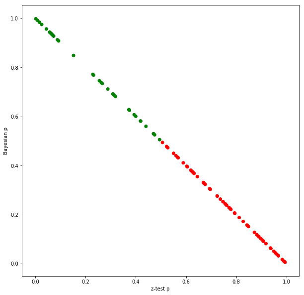
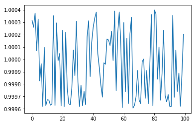
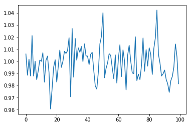
It seems that the two add up to 1. But they don’t add up to 1 exactly, it’s just an approximation (using the exact closed-form Bayesian evaluation, not the MC):

results = run_simulations(funnels, N, num_simulations)
plt.plot([x[1]+x[2] for x in results])

What’s going on here? One of the things every data scientist knows is that, if given $p_f$, it doesn’t mean that the probability that the action hypothesis is true is $1-p_f$.

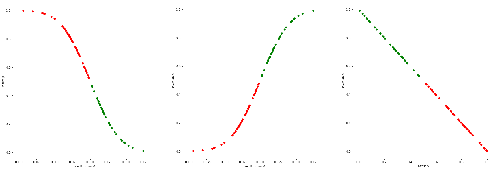
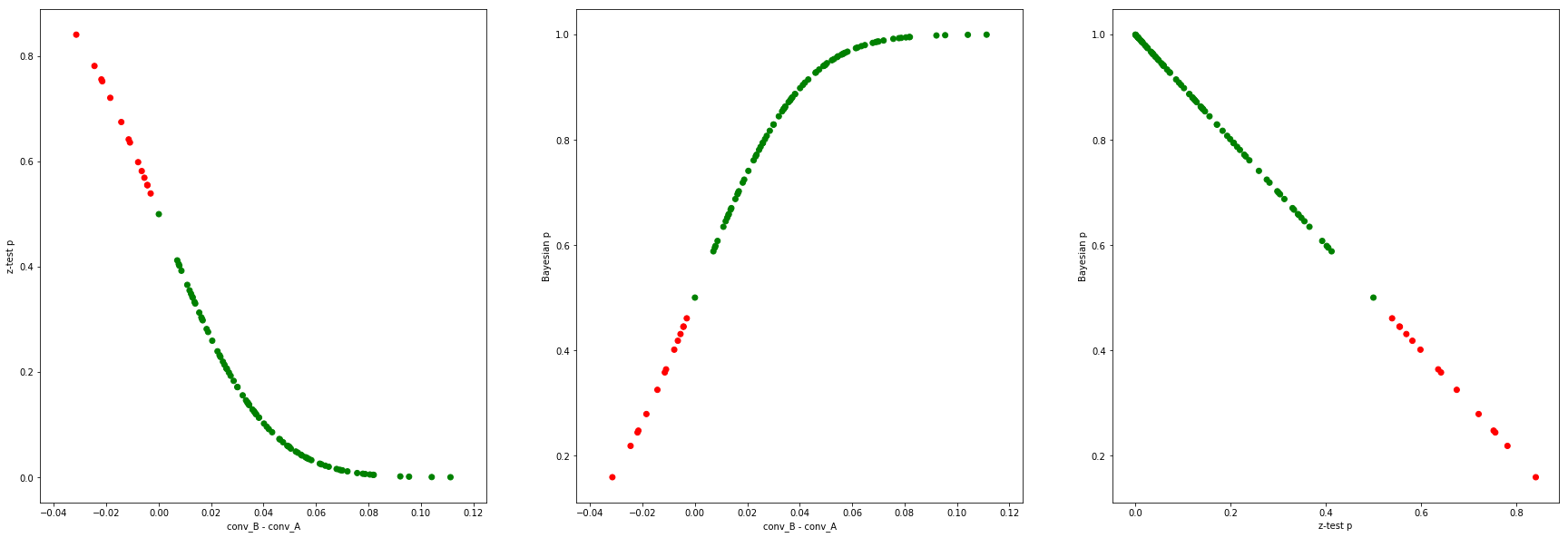
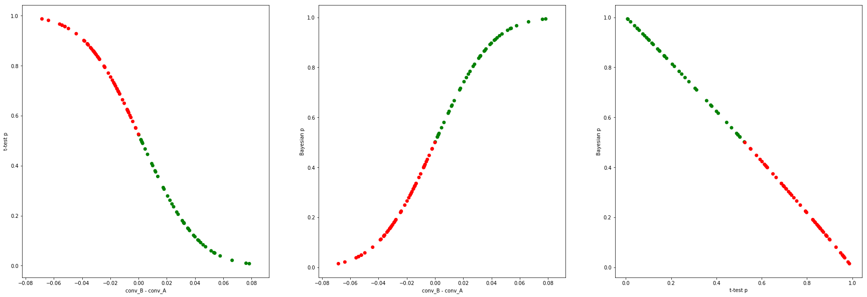
Let’s repeat the above experiment, but with different $N$ sample sizes, different conversions, and also look at cases when the action hypothesis is actually true (funnel B is in fact better). Green dots are cases when the outcome of the experiment was such that B’s conversion was better than A (irrespective of the true conversions), red the opposite, for easier readability. In all cases, 100 A/B tests are performed, and the results are plotted.

$N=1000$, A and B are both 50%:

funnels = [
    [[0.50, 0.50], 0.5], # the first vector is the actual outcomes,
    [[0.50, 0.50], 0.5], # the second is the traffic split
]
N = 1000

$N=1000$, B’s conversion is better than A’s (53% vs 50%):

funnels = [
    [[0.50, 0.50], 0.5], # the first vector is the actual outcomes,
    [[0.47, 0.53], 0.5], # the second is the traffic split
]
N = 1000

In this case, we’re sampling the same curves, but in the region where B’s conversion is better than A’s (more green dots in the green section of the curve).

$N=10,000$, A and B are both 1%:

funnels = [
    [[0.99, 0.01], 0.5], # the first vector is the actual outcomes,
    [[0.99, 0.01], 0.5], # the second is the traffic split
]
N = 10*1000

The equation $p_f + p_b \simeq 1 $ seems to hold in all these cases!

Explanation

With the Z-test, we assume that the Central Limit Theorem (CLT) holds, and model the standard error of the mean (the mean is the conversion) of each funnel with a normal variable $N$, centered on the measured conversion $\mu$, and variance $\sigma^2 = \mu * (1 - \mu) / N$. The difference in conversion is also a normal variable, $N = N_B - N_A$, this has mean $\mu = \mu_B - \mu_A$ and variance $\sigma^2 = \sigma_A^2 + \sigma_B^2$. Then we assume the null hypothesis is true, and calculate the probability of getting at least as extreme results as observed (wrt conversion difference), so we take the integral of the normal from 0 to $\infty$.

With the Bayesian model, we model the actual conversion parameter with a Beta distribution. As long as the $Beta(\alpha, \beta)$ distribution and the $N(\mu, \sigma^2)$ are close enough (with $\mu = \frac{ \alpha }{ \alpha + \beta } $), the two probabilities will be complementary, since in the Bayesian framework we’re computing the complimentary probability. Let’s compare some Beta and normal distributions under with different sample sizes and conversions to check how close these distributions are:

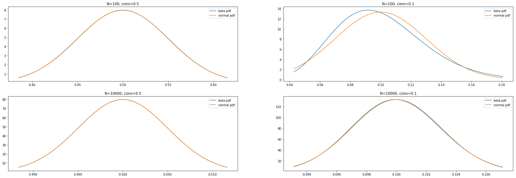
Thanks to the CLT, the only time when the Beta pdf and the normal pdf are noticably different is when we’re close to 0 or 1 in conversion probability, and we’re at low sampe sizes $N$ (top right case, above). We can visualize this directly:

funnels = [
    [[0.90, 0.10], 0.5], # the first vector is the actual outcomes,
    [[0.90, 0.10], 0.5], # the second is the traffic split
]
N = 100

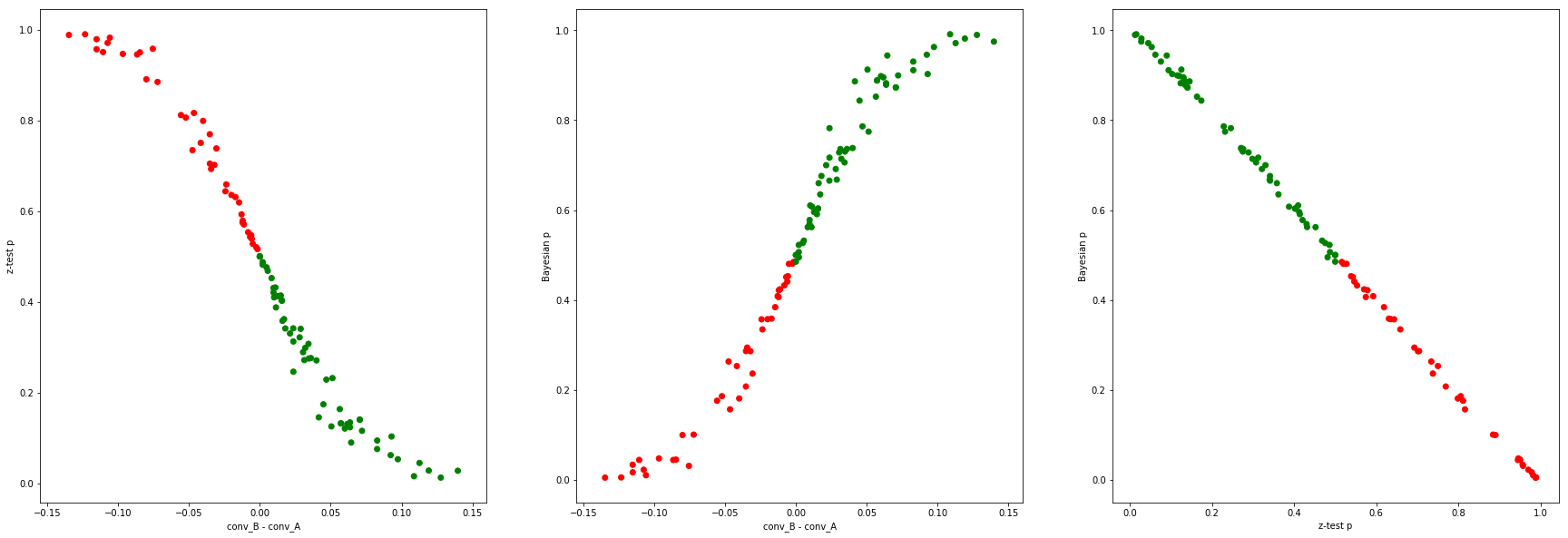
There is now a noticable spread in the curves, and the “error” in the $p_f + p_b \simeq 1$ line goes as high as 0.04:

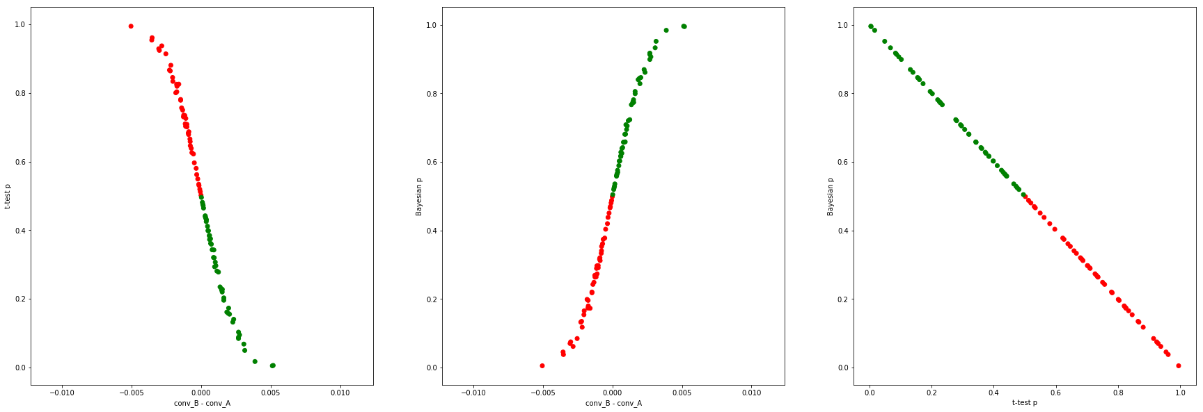
In earlier posts I showed that at moderate $N$ the t-test and the z-test quickly become the same thing, so exchanging the z-test for the t-test doesn’t make a difference.

Bayesian Beta modeling vs the frequentist Fisher’s exact test

Let's do the same, but instead of using the Z-test, let's use Fisher's exact test (which doesn't have a normal distribution assumption) to get the frequentist $p_f$.

funnels = [
    [[0.50, 0.50], 0.5], # the first vector is the actual outcomes,
    [[0.50, 0.50], 0.5], # the second is the traffic split
]
N = 20

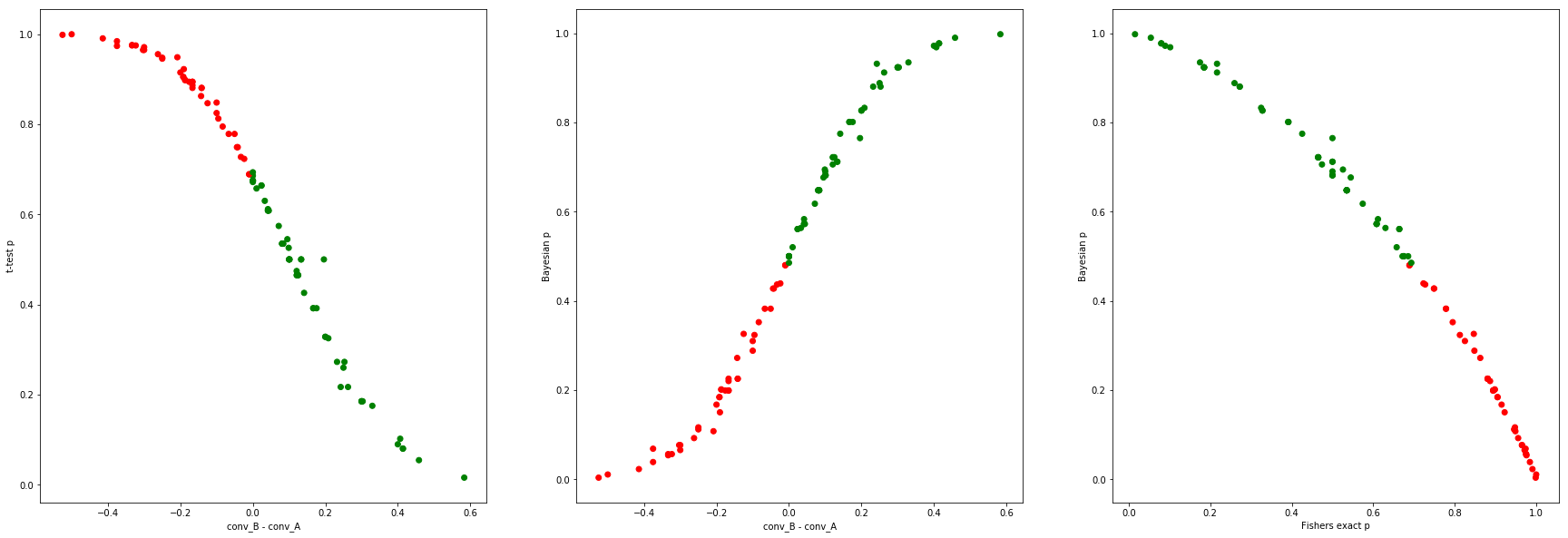
... and the same at $N=1000$:

At high $N$, $p_f + p_b \simeq 1$ also approximately holds, since here all these frequentist tests become the Z-test.

Question: why the concave relationship at low $N$?

Bayesian modeling with normals, priors

There is no set rules for how to perform Bayesian modeling, it is the modeler's choice. It is up to us what kind of distributions we use to model the conversion parameter for our funnels. For example, another popular choice (other than the Beta) is the normal distribution. It goes without saying that if we did that, with the parameters chosen as mentioned above for the z-test, we could get exactly complementary probabilities.

Another choice we have in Bayesian modeling is the prior. The prior is some up-front belief we have about the distribution of the conversions, which we then update based on the outcome of the experiment to get the posterior distribution. Two popular choices are $Beta(1, 1)$, which happens to be the uniform distribution, and $Beta(0.5, 0.5)$, called the Jeffreys prior:

# common priors
plt.figure(figsize=(10,5))
x = np.linspace(0.01, 0.99, 1000)  
plt.plot(x, beta.pdf(x, 1, 1))
plt.plot(x, beta.pdf(x, 0.5, 0.5))
plt.legend(['Beta(1, 1)', 'Beta(0.5, 0.5)'])

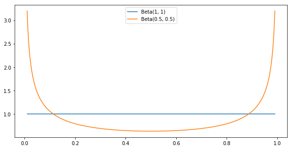
When we have a prior belief expressed as a Beta distribution $Beta(\alpha_0, \beta_0)$, after we run the A/B test which yields $\alpha$ conversions and $\beta$ non-conversion events, the posterior will be the Beta distribution $Beta(\alpha_0+\alpha, \beta_0+\beta)$. As you can imagine, at reasonable samples sizes such as $N>100$, Beta priors with relatively low parameters don’t matter much; this is called “washing out the prior with observations”.

However, note that any sort of prior can be chosen, including a very strong one that doesn’t wash out with $N=1000$ samples, like $Beta(1M, 1M)$; this is saying the modeler has a very strong prior belief that the conversion is 50%, and she needs to see millions of observations to convince her otherwise; getting 10 out of 100 will not convince her, since $Beta(1M+10, 1M+100) \simeq Beta(1M, 1M)$ is still a peak around 0.5 (notice the x-axis):

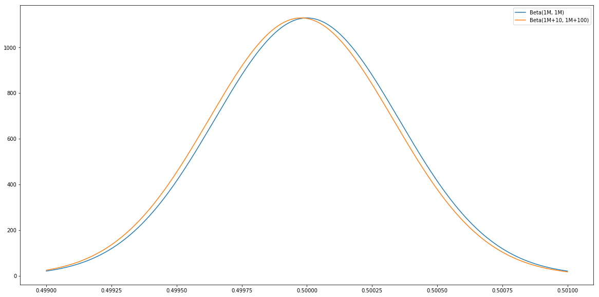
This is a modeling decision. Obviously, with strong priors like this $p_f + p_b \simeq 1$ will not hold (since $p_b$ will be frozen until a lot of observations are collected). Also, any distribution can be chosen by the modeler for the posterior.

Conclusion

So in general, the $p_f + p_b \simeq 1$ approximation is not true, it only happens to roughly hold when:

• using Z-tests on the frequentist side (or other tests whose p value becomes the Z-test's at large $N$), and
• using Beta distributions (or other distributions that become roughly normal at large $N$) for Bayesian modeling, and
• using a weak prior that is washed out

Turning it around: Bayesian inference, when applied to A/B testing using Beta distributions (or other distributions that become normal at large $N$) and weak priors, at reasonable sample sizes, yields roughly complementary probabilities to frequentist tests such as the Z-test (or other tests whose p value becomes the Z-test's at large $N$): $p_f + p_b \simeq 1$. At the end of the day, in conversion A/B testing, in the absence of strong prior beliefs, at reasonable sample sizes we end up putting roughly gaussian shaped functions around measured averages, so different statistical procedures yield roughly the same (complementary) probabilities and decisions.