Exploring prior beliefs with MCMC

Introduction

In the previous post Food deliveries, Bayes and Computational Statistics a first principles simulation was used to calculate the Bayes posterior probability of UberEats being the most popular food delivery service. After I finished writing the post my I was left feeling unsatisfied: I wrote too much simulation code. I realized I could've used a Markov Chain Monte Carlo (MCMC) framework to get the same result with less code. The notebook is up on Github.

So let's do that. Let's use PyMC3, the standard MCMC library for Python. This code is so simple, without further ado, here it is:

import pymc3 as pm
%matplotlib inline

data = {
    'Carriage':  2,
    'Talabat':   2,
    'UberEats':  16,
    'Deliveroo': 12,
}

def uniform_prior(k):
    rs = [pm.Uniform('raw%s' % i, 0, 1) for i in range(k)]
    s = sum(rs)
    return [pm.Deterministic('p%s' % i, rs[i]/s) for i in range(k)]

def run_model(prior, data):
    with pm.Model() as model:
        vals = list(data.values())
        k = len(vals)
        ps = prior(k)
        multi = pm.Multinomial('multi', n=sum(vals), p=ps, observed=vals)
        trace = pm.sample(draws=10*1000, progressbar=True)
        return pm, trace

pm, trace = run_model(uniform_prior, data)

Okay, what's happening here? PyMC3 is an MCMC library, and computes representative samples of random variables based on some data. We specify a model, which is essentially a way to compute a desired random variable (RV) (essentially a probability distribution function, pdf) from other random variables. In this case, we say that multi is a multinomial RV, with the parameters of multi itself being RVs, these are ps in the code. When we specify multi, we pass in our observed values, so we "fix" this RV. The ps RVs are constructed in the prior helper function, named prior because here is where we encode our prior belief about the food delivery business. To match the previous post, we don't assume any courier is more popular than the other, constructed so that the probabilities sum to 1.

When we call sample() on the model, Markov Chain Monte Carlo simulation is performed; the details of this are beyond the scope of this article. The important thing is that after the simulation is complete, trace will contain a sample of all free (non-fixed) RVs, updated according to the observations passed ot the fixed RVs. Ie. when we specified these RVs, we gave our prior belief pdfs, $ p(H) $, whereas trace now contains samples from the posterior pdf, ie. $ p(H|D) $. That's exactly what we worked for in the previous post!

Given this sample that PyMC3 gives us, it's easy to calculate the hypothesis. We simply count the frequency of cases when the probability parameter of UberEats is the maximum in the trace:

hypothesis = [trace['p2'][i] == max([trace['p%s' % j][i] for j in range(k)]) for i in range(len(trace['p0']))]
sum(hypothesis) / len(hypothesis)

The program outputs the probability at 72%, like in the original post.

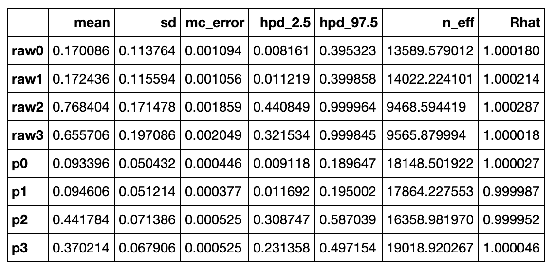
PyMC3 has a few useful helper functions. One is pm.summary(trace), this outputs some statistics about the RVs:

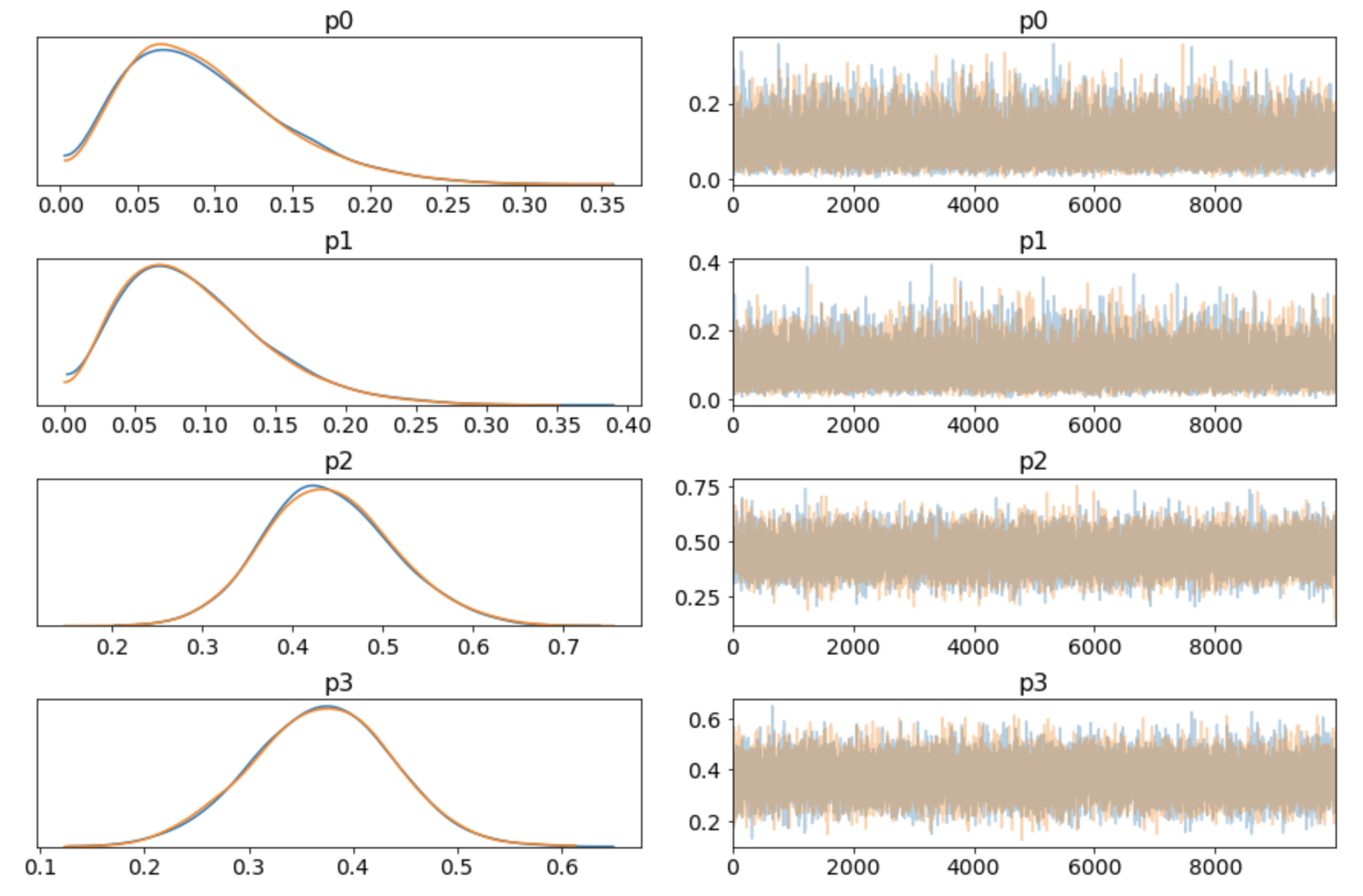
The other is pm.traceplot(trace), this outputs the pdf and the random walk for each RV:

There is something weird here. Looking at the original observation data, half of the deliveries are from UberEats (16/32). The corresponding RV in the summary() output is p2. So why is the posterior mean for p2 0.44 and not closer to 0.50? Intuitively, after looking at the data, shouldn't that be the maximum likelyhood (ML) prediction? Let's think this through:

• the mean is not the ML, but looking at the posterior curve for p2, the maximum of the curve (=ML) is also not at 0.5
• it could be that the simulation has not reached a stationary state (in Markov chain language); but looking at the random walk output, it has (and to double-check I ran it longer, this is not the problem)
• numerical error: this is not the reason

The reason is simple: it's our prior belief. Our prior belief was a uniform distribution. We observed some data and showed it to the model, and based on this our posterior belief was updated, but the prior belief is still baked in. The way to think about this is, the prior pdf slowly morphs into the posterior pdf as data is fed to the model.

One good way to get a feel for this is to imagine feeding a low observation count to the model. Suppose we feed it observations like (1, 0, 2, 1). Should we now believe that Talabat never gets orders? Clearly not.

Another good way to get a feel for this is to feed the model more data, but keeping the same ratios, ie. multiplying each number by 10, like (20, 20, 160, 120). At such high observation counts, the posteriors will be very narrow, and close to the actual ratios. This is called flooding the priors: as the model observes a lot of data, the prior belief is less and less important.

Also the hypothesis probability of UberEats being the most popular will be 98.7%, or almost certain.

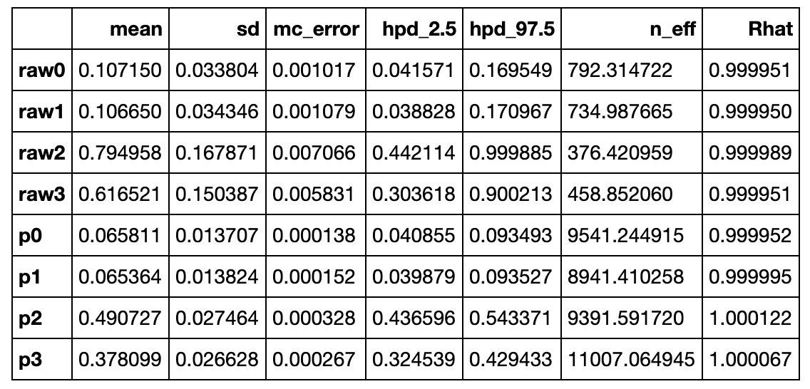
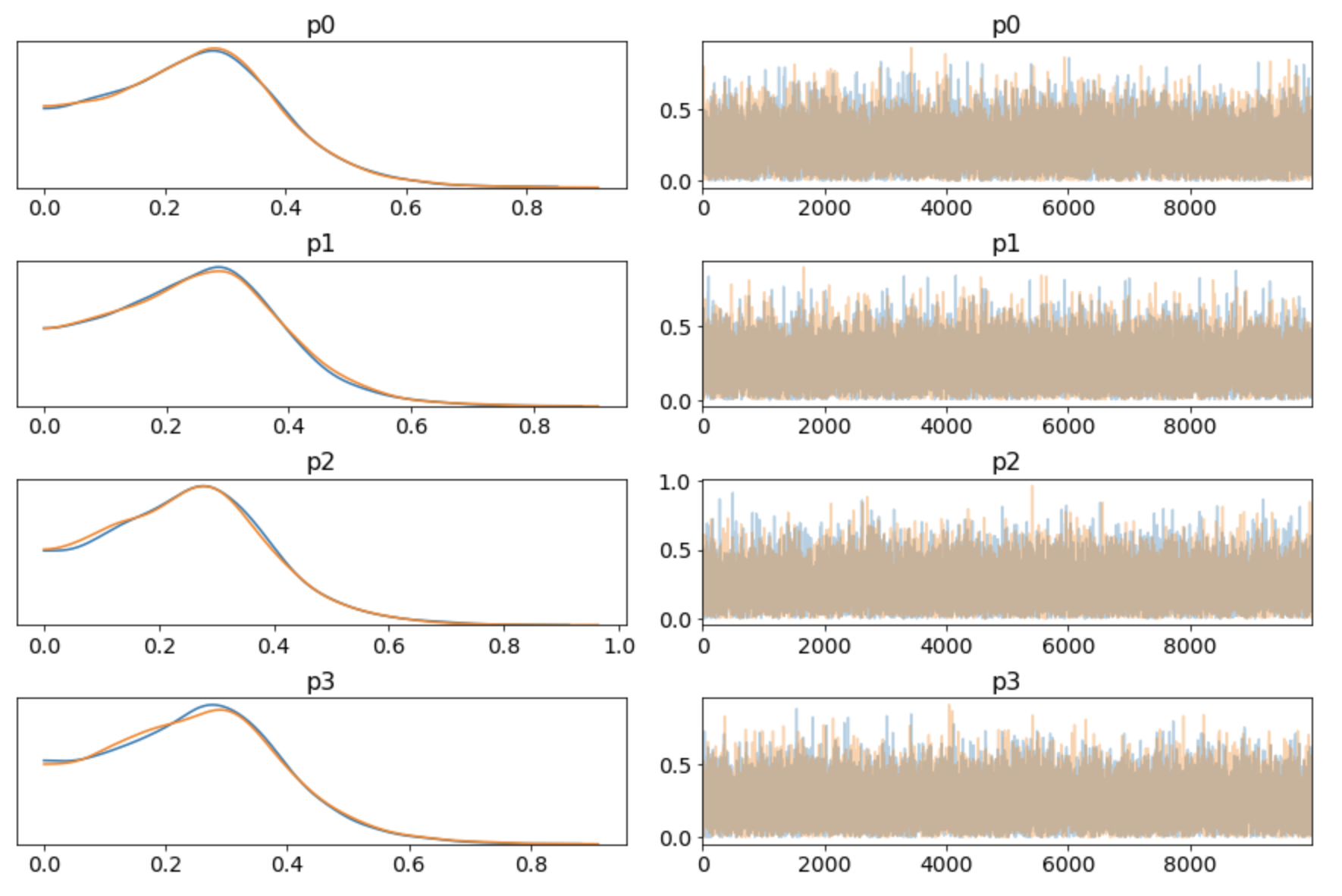
PyMC3 also allows us to easily explore other prior beliefs. For example, we could specify a prior centered around the observed ratios. BAKING OBSERVATIONS INTO THE PRIOR IS A MODELLING MISTAKE, DON'T DO THIS. I just used it as a debugging exercise to make sure that in such a case the posteriors are what I expect them to be, they remain centered on the observed ratios (yes). The evilness also comes out in the function signature, passing the observed values to the prior shouldn't happen. But in any case, it shows how easy it is to change the priors with PyMC3:

def beta_prior(vals, k):
    rs = [pm.Beta('raw%s' % i, vals[i], sum(vals)-vals[i]) for i in range(k)]
    s = sum(rs)
    return [pm.Deterministic('p%s' % i, rs[i]/s) for i in range(k)]

pm, trace = run_model(beta_prior, data)

Going back to the original problem, we can make our code shorter by using PyMC3's built-in Dirichlet distribution. The Dirichlet distribution can be parameterized so that it's the uniform distribution in n-dimenions:

def dirichlet_uniform_prior(k):
    return pm.Dirichlet('ps', a=1*np.ones(k))
pm, trace = run_model(dirichlet_uniform_prior, data)
hypothesis = [ps[2] == max(ps) for ps in trace['ps']]
sum(hypothesis) / len(hypothesis)

Running this reveals something interesting. The probability of the hypothesis that UberEats is the most popular comes out to ~77%, which is about 5% more than before. What's going on here? It turns out that prior we baked in before, although it didn't favor any courier over the others, did have some bias built-in. We sampled each individual raw RV uniformly between 0 and 1, and then divided by the sum. Each raw's mean is 0.5, sum's mean is 2, so the ps component's mean is 0.25. So by constructing the prior like this, we biased it towards (0.25, 0.25, 0.25, 0.25), ie. we said this is a more likely prior than eg. (0.7, 0.1, 0.1, 0.1). This can be seen by using MCMC to just sample:

with pm.Model() as model:
    k = 4
    rs = [pm.Uniform('raw%s' % i, 0, 1) for i in range(k)]
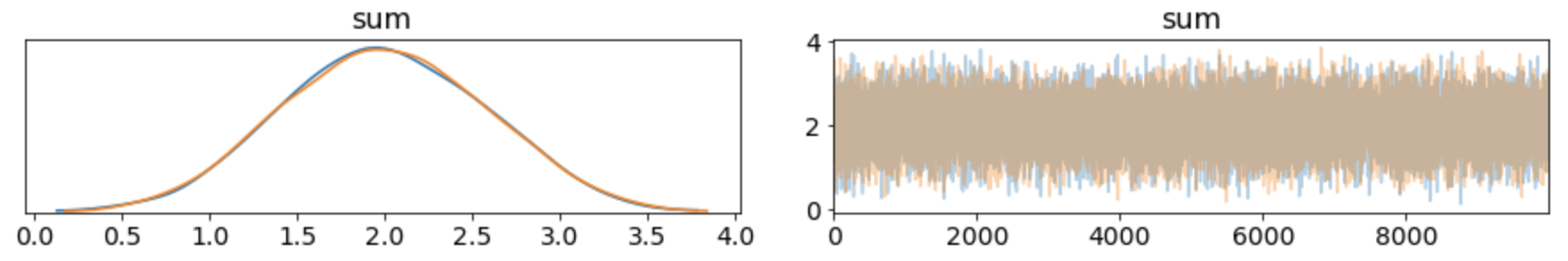
    s = pm.Deterministic('sum', sum(rs))
    [pm.Deterministic('p%s' % i, rs[i]/s) for i in range(k)]
    trace = pm.sample(draws=10*1000, progressbar=True)
    pm.traceplot(trace)

Looking at the sum:

Versus the Dirichlet distribution (see this blog post for more):

with pm.Model() as model:
    k = 4
    pm.Dirichlet('ps', a=1*np.ones(k))
    trace = pm.sample(draws=10*1000, progressbar=True)
    pm.traceplot(trace)

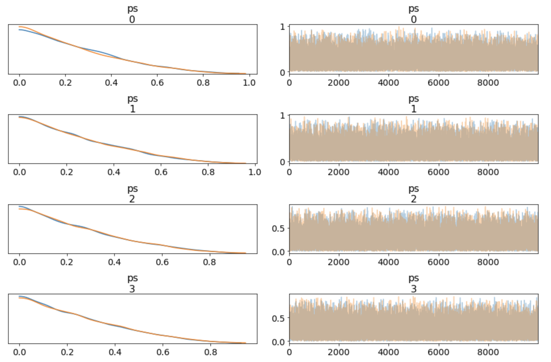
I would say the original post is buggy, because I intended to make no prior assumption (=use the "uninformative prior"), so the Dirichlet distribution (at 𝛼=1) is the right prior.