Food deliveries, Bayes and Computational Statistics

Introduction

I was grabbing a burger at Shake Shack, Mall of the Emirates in Dubai, when I noticed this notebook on the counter. The staff is using it to track food deliveries, and each service (Carriage, Talabat, UberEats, Deliveroo) has its own column with the order numbers. Let's assume this is the only page for the day, and ask ourselves: given this data, what is the probability that UberEats is the most popular food delivery service?. The ipython notebook is up on Github.

This is good challenge to exercise our Bayesian reasoning. Bayes theorem states that $ P(A|B)P(B) = P(A,B) = P(B|A)P(A) $, where $ P(A|B ) $ is the conditional probability of A given B, and $ P(A, B) $ is the joint probability of A and B co-occuring. All we have to do is replace A with H for Hypothesis and B with D for Data, and we get our formula for attacking the challenge: $ P(H|D) = \frac { P(D|H)P(H) }{ P(D) } $. Here Hypothesis is that UberEats is the most popular service, and Data is the observed counts (2, 2, 16, 14) in the notebook.

Simulation

First, let's do a brute-force simulation. Our model is that there are 4 services, each service has an associated probability, the probabilities sum to 1. When a new orders arrives at Shake Shack, it is according to this model that the service is drawn. A single simulation run---given a model (so, 4 probabilities for each service, summing to 1)---consists of 2 + 2 + 16 + 14 = 34 draws, and the outcome is the distribution between the services, eg. (10, 10, 10, 4). In mathematics terms, this drawing is called a multinomial distribution, numpy has a multinomial function, so we will use that. So our outer loops looks something like:

from random import random
from numpy.random import multinomial

data = {
    'Carriage':  2,
    'Talabat':   2,
    'UberEats':  16,
    'Deliveroo': 12,
}

n_models = 1000

def random_model(k):
    ps = [random() for _ in range(k)]
    s = sum(ps)
    return [p/s for p in ps]

def random_simulation(ps, n):
    return list(multinomial(n, ps))

for i in range(n_models):
    model = random_model(len(data.keys()))
    # call random_simulation(model, sum(data.values())) and count things

Since this is a simulation, we had to introduce n_model, the number of random models we sample (the ensemble size). Now we just have to implement the $ P(H|D) $ formula. This is simple. $ P(D|H) $ is the fraction of random_simulation cases that match the data, when the model matches the hypotehesis (see next sentence). $ P(H) $ is the fraction of models (!) that match the hypothesis of UberEats being the most popular, ie. that probability being the highest. $ P(D) $ is the total number of cases when random_simulation matches the data. First, some helper functions:

def same_as_data(outcome):
    return all([i == j for  (i, j) in zip(outcome, list(data.values()))])

def model_satisfies_hypothesis(ps):
    return max(ps) == ps[2] # UberEats

We have to introduce another parameter, the number of trial runs per model, which we'll call n_simulations. The simulation is now (note that this is actually two loops, the list expression for hits is a loop):

n_models = 1000
n_simulations = 1000*1000

hits_total = 0
hits_hypothesis = 0
num_model_satisfies_hypothesis = 0
for i in range(n_models):
    model = random_model(len(data.keys()))
    hits = sum(
        [same_as_data(random_simulation(model, sum(data.values()))) for _ in range(n_simulations)]
    )
    hits_total += hits
    if model_satisfies_hypothesis(model):
        hits_hypothesis += hits
        num_model_satisfies_hypothesis += 1

In terms of these variables:

p_data_given_hypothesis = hits_hypothesis / (num_model_satisfies_hypothesis * n_simulations)
p_hypothesis = num_model_satisfies_hypothesis / n_models
p_data = hits_total / (n_models * n_simulations)
# p_hypothesis_given_data = p_data_given_hypothesis * p_hypothesis / p_data
# but, for better numerics, the above simplifies to:
p_hypothesis_given_data = hits_hypothesis/hits_total

That's it! We just have to run this simulation, and it will tell us our desired probability. Unfortunately, this is actually a lot of random(), calls. On my Macbook, this takes a long time to run. So I modified it a bit, updated and displayed the estimate hits_hypothesis/hits_total as the simulation was running. This is what it looks like:

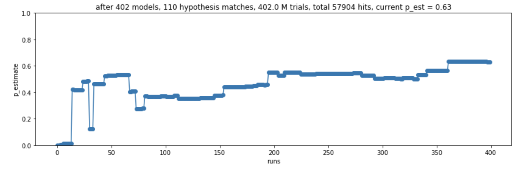
Obviously it takes a long time for the simulation to converge. In fact, the p_est shown in the screenshot above is not correct, the simulation has not yet converged. The reason is that the simulation is sparse. In most cases, there are no hits, so we waste a lot of cycles not updating our estimate hits_hypothesis/hits_total.

Monte Carlo integration

The above code is a good start, but it's terribly inefficient. Actually, there's no reason to brute-force the simulation itself, since there is an explicit formula for the multinomial probability of drawing $ k_i $ given $ p_i $ probabilities. The package scipy implements it, it's also called multinomial (like the numpy one), but this is the explicit probability mass function, not a random draw. Actually all we have to do is replace one line, the hits calculation, to compute the fractional probability of observing the data. It changes the meaning of the variables (the hits variables are no longer integers counts, instead they're summed fractions), but the ratios are the same. So the simulation becomes:

from random import random
from scipy.stats import multinomial

data = {
    'Carriage':  2,
    'Talabat':   2,
    'UberEats':  16,
    'Deliveroo': 12,
}

n_models = 100*1000

def random_model(k):
    ps = [random() for _ in range(k)]
    s = sum(ps)
    return [p/s for p in ps]

def same_as_data(outcome):
    return all([i == j for  (i, j) in zip(outcome, list(data.values()))])

def model_satisfies_hypothesis(ps):
    return max(ps) == ps[2] # UberEats

hits_total = 0
hits_hypothesis = 0
num_model_satisfies_hypothesis = 0
for i in range(n_models):
    model = random_model(len(data.keys()))
    hits = multinomial(sum(data.values()), model).pmf(list(data.values())) # <-- this changed
    hits_total += hits
    if model_satisfies_hypothesis(model):
        hits_hypothesis += hits
        num_model_satisfies_hypothesis += 1
p_hypothesis_given_data = hits_hypothesis/hits_total
print(p_hypothesis_given_data)

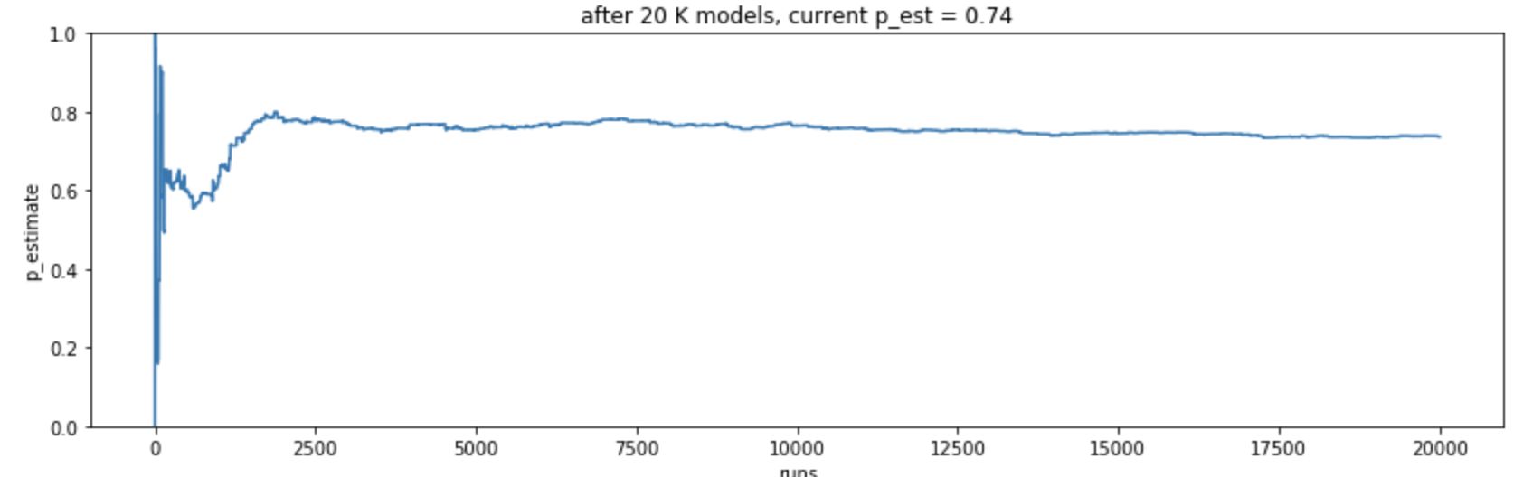
Note that we now no longer need the variable n_simulations. This is now lighting fast, converges in a few seconds, and quickly tells us that the probability we're looking for is 72%. Given what I saw on the notebook, the probability that UberEats is their most popular delivery service is ~72%. Given this code, it's easy to check another one. What's the probability that Deliveroo is the most popular? Just change model_satisfies_hypothesis, run it again, and it's ~28%. The other two have almost zero chances of actually being the most popular. In this whole discussion I'm assuming a uniform prior, ie. I have no prior bias towards believing one service being more popular than the rest.

Note: this post has a subtle bug in the prior assumption. For more, see this subsequent post. The prior, as implemented above, does not favor one courier over another, but it is not in fact uniform in p-space.

Before moving on, here's a screenshot of this version, but before it converges. It shows the initial oscillations, which is what we were observing with the brute-force simulations (note that it eventually converges to 0.72):

Integrals

In case you remember college calculus, what we're doing above is a Monte Carlo (MC) integration of:

$$ \frac { \int_{\sum p_i = 1 \wedge p_3 = max(p_i)} P(x_i=k_i) dp_i }{ \int_{\sum p_i = 1} P(x_i=k_i) dp_i } $$

where:

$$ P(x_i = k_i) = \frac {N!}{x_1! ... x_s!} p_1^{x_1} ... p_s^{x_s} $$

is the multinomial probability mass function evaluated at

$$ k_i = (2, 2, 16, 14), s = 4, i = 1.. 4, N = \sum k_i = 34.$$

It's called Monte Carlo because instead of computing the integral explicitly, we're taking random samples in p-space and using that to estimate. The $ P() $ function above can be integrated, it's just a polynomial, and the whole integral can be explicitly calculated (I think) with pen and paper (or Mathematica); both numerator and denominator constraints are a hyperplane in 4D p-space, with the numerator being more tricky because of the $ max() $ constraint. I will let the reader do this as homework :)

If you're having trouble understanding this post, check out the free book Think Bayes.