Breaking Bell's Inequality with Monte Carlo Simulations in Python
Marton Trencseni - Sun 01 September 2024 - Physics
Introduction
In this article, we explore a game that challenges the very foundations of classical physics and introduces us to the strange world of quantum mechanics. The game involves three players — Alice, Bob, and Victor — who perform a series of experiments to test a fundamental principle known as Bell's theorem. By carefully selecting their measurement devices and analyzing the outcomes, Alice and Bob aim to determine whether the physical world can be explained by deterministic local hidden variables. Through Monte Carlo Python simulations, we will see how classical strategies adhere to Bell's inequality, and how to break it using non-local action-at-a-distance and entangled qubits. The code is up on Github.
Bell game
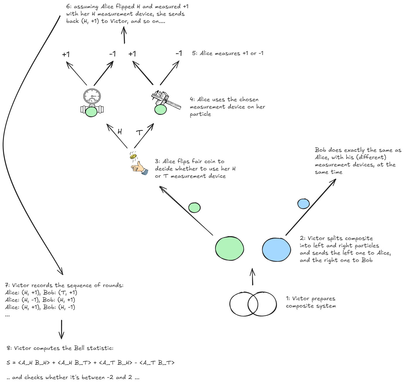
Imagine a game — let's call it the Bell game — involving three players: Alice, Bob, and Victor. Alice and Bob are situated in two distant locations, far enough apart that no signal — not even light — could travel between them in the time it takes to perform a single round of the game. Their colleague, Victor, prepares a pair of particles, the left particle and the right particle, and sends them to Alice and Bob, respectively. The particles may be classical objects like coins, dice, apples, or, bits recorded on digital storage, or, intriguingly, quantum particles such as entangled photons, which can be modeled as qubits. Before the game, Victor tells Alice and Bob what kind of particles he will send, and Alice and Bob can agree between each other what measurement devices to use. Once the game starts, the choice of measurement devices is fixed.
Upon receiving their respective particles, Alice and Bob each perform one of two possible measurements. Alice chooses between two measurement devices, which we will call $A_H$ (for Heads) and $A_T$ (for Tails). Similarly, Bob also chooses between two measurement devices, $B_H$ and $B_T$. Both Alice and Bob flip a fair coin to pick their measurement devices, which means the 4 cases $HH$, $HT$, $TH$ and $TT$ are all equally like at $p=1/4$. Each measurement results in a binary outcome: either $+1$ or $-1$.
The key assumption underlying the classical view of this experiment is that the properties of the particles — the hidden variables — determine the outcomes of these measurements. If Alice measured $A_H$ and obtains the result $+1$, it is assumed that the particle she received already carried a hidden property corresponding to $+1$ for the measurement $A_H$. Likewise, if Bob measures $B_T$ and gets $-1$, then his particle must have had a hidden property corresponding to -1 for $B_T$.
At the end of each round, both Alice and Bob send back to Victor two pieces of information each: whether they flipped $H$ or $T$, and what their measurement outcomes was, $+1$ or $-1$. Victor records 4 pieces of binary information: (Alice flipped $H$ or $T$, Alice measured $+1$ or $-1$, Bob flipped $H$ or $T$, Bob measured $+1$ or $-1$). The game is played repeatedly over a large number $N$ of rounds, and Victor ends up with an $N$ long list of records. Per the above consideration, each combination $HH$, $HT$, $TH$ and $TT$ will occur about $N/4$ times.
The full game is depicted below:
Bell statistic
The goal of the game is to compute a special mathematical quantity called the Bell statistic, which quantifies the correlation between the measurement outcomes of Alice and Bob. This statistic is calculated over a large $N$ number of rounds, as follows:
$ S = \langle A_H B_H \rangle + \langle A_H B_T \rangle + \langle A_T B_H \rangle - \langle A_T B_T \rangle $
Here, each term represents a product of Alice's and Bob's measurement outcomes, averaged over many rounds of the game. For example, $A_H B_H$ is the product of Alice's outcome when she measures $A_H$ and Bob's outcome when he measures $B_H$. The average here is taken over the roughly $N/4$ times when Alice and Bob both flipped H. This can be made more explicit by indexing the averaging operator $\langle \cdot \rangle$ by the cases it is indexing:
$ S = \langle A_H B_H \rangle_{HH} + \langle A_H B_T \rangle_{HT} + \langle A_T B_H \rangle_{TH} - \langle A_T B_T \rangle_{TT} $
For large $N$, the 4 cases $HH$, $HT$, $TH$ and $TT$ will occur roughly at the same frequency $N/4$, so each of the term counts will be abpit $N/4$. This means the sum can be rewritten into an overall average:
$ S = 4 \cdot \langle A_H B_H + A_H B_T + A_T B_H - A_T B_T \rangle_{all} $
Now, let's establish a crucial constraint: If the world is governed by deterministic local hidden variables, which assume that the particles’ properties are fully determined by hidden variables existing prior to and independent of measurement, then the Bell statistic $S$ is bound to always lie within a certain range. Specifically, if Alice and Bob perform many rounds of this game and compute the $S$ over all trials, the absolute value of this average cannot exceed 2:
$ S \leq 2 $
This is known as a Bell inequality. It captures the essential limitation imposed by any theory based on local hidden variables — theories that adhere to classical notions of determinism (no random chance in the measurement apparatus), locality (no faster-than-light influences) and realism (pre-existing properties).
Relating the game to local hidden variables
Let's explore why this inequality holds for any deterministic local hidden variable theory. The central idea is that if the measurement outcomes are predetermined by hidden variables, then Alice’s and Bob’s choices of measurements and their outcomes cannot affect each other instantaneously. Each particle, upon leaving Victor, carries its own set of hidden variables that dictate the outcomes of Alice's and Bob's measurements.
Consider the combination:
$ a_H b_H + a_H b_T + a_T b_H - a_T b_T $
where $a_H$, $a_T$, $b_H$, and $b_T$ are the predetermined hidden values (either $+1$ or $-1$) that dictate the outcomes for Alice’s and Bob’s measurements. We can simply look through all $ 2^{4} = 16 $ combinations of assigning +1 and -1 to these variables, and see that in all cases, the Bell sum above is always $+2$ or $-2$:
def bell_sum(A_H, A_T, B_H, B_T):
    return A_H*B_H + A_H*B_T + A_T*B_H - A_T*B_T

print('A_H  A_T  B_H  B_T    Bell-sum')
print('------------------------------')
values = [-1, +1]
for A_H, A_T, B_H, B_T in product(values, values, values, values):
    print(f' {A_H:2}   {A_T:2}   {B_H:2}   {B_T:2}    ->    {bell_sum(A_H, A_T, B_H, B_T):2}')
Prints:
A_H  A_T  B_H  B_T    Bell-sum
------------------------------
 -1   -1   -1   -1    ->     2
 -1   -1   -1    1    ->     2
 -1   -1    1   -1    ->    -2
 -1   -1    1    1    ->    -2
 -1    1   -1   -1    ->     2
 -1    1   -1    1    ->    -2
 -1    1    1   -1    ->     2
 -1    1    1    1    ->    -2
  1   -1   -1   -1    ->    -2
  1   -1   -1    1    ->     2
  1   -1    1   -1    ->    -2
  1   -1    1    1    ->     2
  1    1   -1   -1    ->    -2
  1    1   -1    1    ->    -2
  1    1    1   -1    ->     2
  1    1    1    1    ->     2
Note that the Bell sum above is not the same thing as the Bell statistic, which can take on values between $-2$ and $2$.
As a result, if Victor prepares many such pairs and the game is repeated over numerous trials, the average value of this combination will always fall within the range $[-2, +2]$. No matter how Alice and Bob choose their measurements, or what hidden variables Victor might encode in the particles, the Bell inequality holds if local hidden variables govern the experiment.
Simulating the Bell game in Python
To understand Bell's theorem through simulation, let's set up a Python program that models the game between Alice, Bob, and Victor. In this game, Victor prepares a composite system, splits it into two parts (left and right in the code), and sends one part to Alice and the other to Bob. Alice and Bob then perform their measurements $H$ or $T$ based on a coin flip, and we compute the Bell statistic to see if they can violate the Bell inequality:
def bell_experiment(N):
    total = 0
    for _ in range(N):
        # Generate a composite object and split it
        composite = generate_composite()
        left, right = split(composite)

        # Alice's coin flip determines which measurement device she uses
        A_which = flip_coin()
        measure_A = measure_A_H if A_which == 0 else measure_A_T
        A = measure_A(left)

        # Bob's coin flip determines which measurement device he uses
        B_which = flip_coin()
        measure_B = measure_B_H if B_which == 0 else measure_B_T
        B = measure_B(right)

        # Compute the contribution to the Bell statistic
        multiplier = -1 if A_which == 1 and B_which == 1 else 1
        total += multiplier * A * B

    # Calculate the Bell statistic and print the result
    bell_statistic = 4 * float(total) / N
    print(f'Bell Statistic: {bell_statistic:.3}')
To make this work, we have to define the functions generate_composite(), which returns something that van then be split into two parts, left and right, using the split() function. Additionally, we need 4 measurement functions: measure_A_H(), measure_A_T(), measure_B_H(), measure_A_T(). Remember that the measurement functions have to return $+1$ or $-1$. To clarify the setup of the game, it is assumed that both Alice and Bob know what function Victor is using to generate_composite() and split(), and can cooperate with the other to pick what measurement function they use to attempt to break the Bell inequality.
In the simplest case, we can have the measurement functions return a fixed value, like:
def measure_A_H(_):
    return 1

def measure_A_T(_):
    return 1

def measure_B_H(_):
    return 1

def measure_B_T(_):
    return 1
In this trivial case, the particles aren't even needed, we can just use a dummy implementation, like:
def generate_composite():
    return None, None

def split(composite):
    left = composite[0]
    right = composite[1]
    return left, right
We can run the simulation like:
bell_experiment(N=1000*1000)
It will print 2.0. The reader is free to try the other 16 combinations as well, and observe that they do not break the Bell inequality. How about if Victor rolls a dice, and sends the same dice to Alice and Bob?
def generate_composite():
    d = roll_dice()
    composite = (d, d)
    return composite
Now Alice and Bob receive some random number between $1$ and $6$, and they know that the other also received the same.
Let's say Alice's $H$ function cuts the range in half, and her $T$ function checks for parity and Bob does the same:
def measure_A_H(q):
    result = 1 if q <= 3 else -1
    return result

def measure_A_T(q):
    result = 1 if q % 2 == 0 else -1
    return result

measure_B_H = measure_A_H
measure_B_T = measure_A_T
Running bell_experiment(N=1000*1000) prints -0.665. We can also try Bob doing the opposite:
measure_B_H = measure_A_T
measure_B_T = measure_A_H
Running bell_experiment(N=1000*1000) prints 2.0. These are just examples, the point is that in these cases Victor introduces randomness (in this example, by using roll_dice()), Alice and Bob both get the same thing, their measurement functions are deterministic (don't use randomness) and local (don't peek at what the other is doing), and they cannot break Bell inequality, however we change the code.
Let's see what happens if Victor also randomly changes what he sends to Alice and Bob. He rolls a dice, if its less than or equal to $4$, both Alice and Bob get the same result. But if it's 5 or 6, Alice gets the value, but for Bob he sends 5 or 6 based on a coin flip. So if Alice and Bob get a value less than or equal to $4$, they know the other has the same, but if they get 5 or 6, the other may have the other one. So the values are not always identical, but correlated. In code:
def generate_composite():
    d = roll_dice()
    composite = (d, d if d <= 4 else flip_coin(heads=5, tails=6))
    return composite
Again, we can try various measurement functions for Alice and Bob, for example:
def measure_A_H(q):
    result = 1 if q <= 4 else -1
    return result

def measure_A_T(q):
    result = 1 if q % 2 == 0 else -1
    return result

measure_B_H = measure_A_H
measure_B_T = measure_A_T
Running bell_experiment(N=1000*1000) prints 0.33. Switching Bob's functions prints 1.67. As before, these are just examples, but they demonstate that Alice and Bob cannot break the Bell inequality.
Random measurement functions
One last thing we could try is introducing randomness into the measurement functions. In the cases above, they always took their portion of the composite Victor constructed (left or right), and the Python code was completely deterministic, a series of if statements. If we do this, we no longer deterministic, the first word in "deterministic local hidden variable theory". But, even with randomness, Alice and Bob cannot break the Bell inequality. We can try this like:
def generate_composite():
    d = roll_dice()
    composite = (d, d if d <= 4 else flip_coin(heads=5, tails=6))
    return composite

def measure_A_H(q):
    result = 1 if q <= 4 else -1
    return result

def measure_A_T(q):
    result = 1 if q % 2 == 0 else -1
    return result

measure_B_H = measure_A_T

def measure_B_T(q):
    result = flip_coin(heads=1, tails=-1) # <----------- randomness at Bob
    return result
Running bell_experiment(N=1000*1000) prints 0.66. We can try all sorts of other versions, but we won't be able to break the Bell inequality.
Breaking the Bell inequality with non-local information
So far it seems like our initial argument stands: we said that there are $16$ combinations of $+1$ and $-1$ outcomes for the measurement outcomes, and all are either $+2$ or $-2$, and so the average has to be between $+2$ and $-2$. The way to break it is to condition the measurement value of one of the players on the other's. For example, in our code, Bob's measurement functions will check whether Alice used $A_H$ or $A_T$, and what the measurement result was ($+1$ or $-1$), and conditions the return based on that. This means that in our simulation Bob's measurement accesses Alice's measurement, which, per our initial assumption is not possible since they are far apart (there is not enough time for light to arrive from one to the other per round). But, we can still simulate this seemingly non-physical scenario in Python code. First, we change the particle creation code, and simulate action-at-a-distance (like a "worm hole"), that allows the left and right particles to see each other:
def generate_composite():
    d = roll_dice()
    composite = (d, d if d <= 4 else flip_coin(heads=5, tails=6))
    return composite

def split(composite):
    left  = {'value': composite[0]}
    right = {'value': composite[1]}
    # we enable both left and right parts to peek at each other
    # in physics, this is called action-at-a-distance
    left['other'] = right
    right['other'] = left
    return left, right
Let's have Alice use her usual measurement devices, but let's have the particle remember which measurement happened — this in itself does not break any of our assumptions. In code:
def measure_A_H(q):
    # the particle remembers which measurement was performed and what the result was
    # in itself, this is not cheating
    q['measure'] = 'H'
    q['result'] = 1 if q <= 4 else -1
    return q['result']

def measure_A_T(q):
    q['measure'] = 'T'
    q['result'] = 1 if q['value'] % 2 == 0 else -1
    return q['result']
Bob's measurement apparatus will use action-at-a-distance and peek at what happened at Alice's side:
def measure_B_H(q):
    # always return what Alice measured
    q['result'] = q['other']['result']
    return q['result']

def measure_B_T(q):
    # condition on which measurement Alice performced and use her result
    q['result'] = q['other']['result'] if q['other']['measure'] == 'H' else -1*q['other']['result']
    return q['result']
Running bell_experiment(N=1000*1000) prints 4.0. We broke the Bell inequality!
What happened here? Because $B_H$ always returns what Alice measured, these $ A B $ products will always be $+1$ in the Bell sum. In $B_T$, if Alice measured $A_H$, we return the same, again in this case the $ A B $ products will be $+1$, and in the $A_T$ case, we return Alice's result multiplied by -1. So in the $A_T B_T$ case the $ A B $ product will be $-1$, but remember that in the Bell statistic this term has a $-1$ multiplier in front (the last term):
$ S = \langle A_H B_H \rangle + \langle A_H B_T \rangle + \langle A_T B_H \rangle - \langle A_T B_T \rangle $
So, by accessing the other's measurement results instantly, which in Physics is called action-at-a-distance, we are able to force the Bell sum $S$ to be like:
$ S = 1 + 1 + 1 - (-1) = 4 $
This is only possible with action-at-a-distance, since otherwise Bob does not know whether Alice is using her $A_H$ or $A_T$ measurement device, so even if Bob flipped $T$ and knows what her particle is (because let's say they're identical, like in the earlier cases), he doesn't know what to do, because he doesn't know whether Alice used her $H$ or $T$.
Now, here's where things get interesting: what about our physical reality? Can any sort of composite system prepared by Victor, then separated—the "left" part sent to Alice, the "right" part sent to Bob—break the Bell inequality, with Alice and Bob being spacelike-separated per round?
Quantum mechanics breaks the Bell inequality
The shocking result is that, Yes, our physical reality breaks the Bell inequality!.
Victor can prepare a pair of quantum particles in a special state known as an entangled state. In this state, the outcomes of Alice's and Bob's measurements are not just random but are correlated in a way that defies any classical explanation based on local hidden variables. Remarkably, quantum mechanics predicts that the Bell statistic can exceed the classical bound of $2$. In fact, it can reach up to $2\sqrt{2} \approx 2.828$, a limit known as the Tsirelson bound. So it cannot get all the way up to $4$, like our toy Python example, but it does break $2$.
In this scenario Victor takes $2$ electrons (or $2$ photons), each of which can be modeled as a $2$-state quantum object, a qubit. He takes these $2$ qubits, and prepares them in the so-called anti-aligned singlet state:
$ ( | 01 \rangle - | 10 \rangle )/√2 $
Then, he sends the left qubit to Alice, and the right qubit to Bob. Alice flips her coin, and either uses the Pauli operator $\sigma_z$ or $\sigma_x$ to measure her qubit. Bob flips his coin, and either uses the operator $ -(\sigma_x + \sigma_z)/\sqrt{2} $ or $ (\sigma_x - \sigma_z)/\sqrt{2} $ to measure the second qubit. What this exactly means is will not be clear from this article, but the point is:
- this can be done in practice
- Alice and Bob do not communicate with eather, they are space-like separated in each round
However, because measurements in quantum mechanics have the weird property of action-at-a-distance, in the above scenario, Victor would compute the Bell statistic $2.828$, ie. our physical world breaks the Bell inequality. In other words, quantum mechanics cannot be decribed by a deterministic, local hidden variable theory. The below Python code simulates this scenario, and because quantum mechanics has action-at-a-distance, we have to keep our seemingly unphysical "other" references in our particles, and our measurement functions have to peek:
def generate_composite():
    # we generate pairs of particles with anti-aligned spins in the singlet state
    # the line of code below doesn't matter, it's just for documentation
    return {'state': '(|01>-|10>)/√2'}
    # |0> is the eigenstate of the Pauli operator σ_z corresponding to eigenvalue (=measurement outcome) +1
    # |1> is the eigenstate of the Pauli operator σ_z corresponding to eigenvalue (=measurement outcome) -1
    # |+> is the eigenstate of the Pauli operator σ_x corresponding to eigenvalue (=measurement outcome) +1
    # |-> is the eigenstate of the Pauli operator σ_x corresponding to eigenvalue (=measurement outcome) -1
    # the above state can be rewritten in terms of |+> and |->, like:
    # (|01>-|10>)/√2  =  (|-+>-|+->)/√2

def split(composite):
    # in quantum mechanics, there is no sense to talk about a left and right
    # value (before measurement) of a singlet composite system..
    left  = {'value': None}
    right = {'value': None}
    # we enable both left and right parts to peek at each other
    # in physics, this is called action-at-a-distance
    left['other'] = right
    right['other'] = left
    return left, right

def measure_first_qubit(q, orientation):
    q['measure'] = orientation
    # Alice measures using σ_z or σ_x
    # in both cases, the amplitudes of the 2 possible states are equal = 1/√2,
    # so the probability of both measurement outcomes is 1/2
    # but the post-measurement state is not the same in the 4 cases (2 measurements, each 2 outcomes ±1
    # if Alice uses σ_z and measures +1 on the first qubit, the post measurement state of the composite system is |01>
    # if Alice uses σ_z and measures -1 on the first qubit, the post measurement state of the composite system is |10>
    # if Alice uses σ_x and measures +1 on the first qubit, the post measurement state of the composite system is |+->
    # if Alice uses σ_x and measures -1 on the first qubit, the post measurement state of the composite system is |-+>
    q['result'] = flip_coin(heads=1, tails=-1)
    return q['result']

measure_A_H = lambda q: measure_first_qubit(q, 'H') # Alice uses the Pauli operator σ_z to measure the first qubit
measure_A_T = lambda q: measure_first_qubit(q, 'T') # Alice uses the Pauli operator σ_x to measure the first qubit

p = 1/(4-2*sqrt(2))
def measure_second_qubit(q, orientation):
    # Bob's H corresponds to using the operator -(σ_x+σ_z)/√2 to measure the second qubit
    # Bob's T corresponds to using the operator  (σ_x-σ_z)/√2 to measure the second qubit
    # the math here is straightforward quantum theory:
    # let's look at an example:
    # suppose Alice flipped a coin and used σ_z (which we labeled Alice's H) and measured +1 on the first qubit, leaving the composite system in the state |01>
    # suppose that now Bob flips a coin and uses -(σ_x+σ_z)/√2 (which we labeled Bob's H):
    # the challenge now is to express the composite state |01> in terms of the eigenvectors of Bob's measurement operator -(σ_x+σ_z)/√2
    # suppose the 2 eigenvectors are U and V with eigenvalues +1 and -1, and we can write |01> = u*|U> + v*|V>, where u and v are the complex amplitudes
    # this can be done on a piece of paper, to find u, v, U, V, and then the probabilities of outcome +1 is p=u^2 and -1 is 1-p=v^2=1-u^2
    # .. where p is the number defined above p = 1/(4-2*sqrt(2)), because I did the math on paper
    # there are 16 combinations of Alice and Bob measurements and outcomes (2 people, each 2 measurements, each measurement 2 outcomes)
    # .. which can be neatly written into a table, and the probability is always p or 1-p
    # see:
    #     https://docs.google.com/spreadsheets/d/1MfsGAqPoN1gK5iA3veipgoaSQ_mhqOL4bLhfYCqy_Sk
    #
    # the code below encodes this table
    q['measure'] = orientation
    sign = 1 if orientation == 'H' or q['other']['measure'] != orientation else -1
    if q['other']['result'] == 1:
        q['result'] = sign * flip_coin(p, 1, -1)
    else:
        q['result'] = sign * flip_coin(p, -1, 1)
    return q['result']

measure_B_H = lambda q: measure_second_qubit(q, 'H')
measure_B_T = lambda q: measure_second_qubit(q, 'T')
Running bell_experiment(N=1000*1000) prints 2.82. Note that this code just simulates quantum mechanics, in the sense that in this simulation, it returns the measurement outcomes $+1$ and $-1$ with the correct probabilities, but it's not simulating a qubit in essence — only a qubit in a quantum computer can simulate another qubit.
Explanation
I will not provide the derivation of the quantum mechanicalal probabilities, but will simply give the table of values. The key is that the conditional probabilities of Bob measuring $+1$ or $-1$ with his $H$ and $T$ devices, given whether Alice used $H$ or $T$ and measured $+1$ or $-1$ is given by this table, where $ p = 1/(4-2\sqrt{2}) \approx 0.8535 $. Deriving this table is relatively easy, a talented college physics student can do it, I did it with pen and paper:
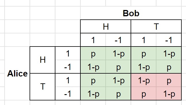
So, for example, if Alice flips $H$ and measures $+1$, and Bob flips $H$, then he will measure $+1$ with probability $p$, and measure $-1$ with probability $1-p$. The Python code above encodes this table in an efficient way. The key here is that the measurement outcomes of Bob in the world of quantum mechanics depends on both:
- which device Alice used
- what the measurement outcome of Alice was
Note that the second point is not action-at-a-distance in itself, since even in the classical case, Bob's measurement outcome can be correlated with Alice — for example, in one of the examples above, Victor sent the same particle to both, and both can use the same devices, so their measurements will be identical — so Bob will always know what Alice's outcome is for both measurement, but he won't know which one she measured.
Notice that the probability matrix is symmetrical, so it doesn't matter whether in our simulation Alice goes first, and then Bob measures, or vica versa. This makes sense, since in the physical situation we're simulating, Alice and Bob are space-like separated, so physically there is no sense to say which of them goes first.
Also note that the probability matrix has four 2x2 sub-matrices. The green ones are all identical, while the red one is the transpose of the green one. It is the presence of the red matrix that leads to the violation of the Bell inequality and requires action-at-a-distance. To see this, let's replace the red one with another copy of the green matrix, like:
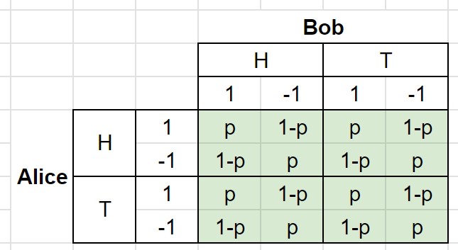
This version no longer required action-at-a-distance, in fact it can be encoded quite simply with hidden parameters by Victor:
p = 1/(4-2*sqrt(2))

def generate_composite():
    A_result = flip_coin(bias=0.5, heads=1, tails=-1)
    if A_result == 1:
        B_result = flip_coin(bias=p, heads=1, tails=-1)
    else:
        B_result = flip_coin(bias=1-p, heads=1, tails=-1)
    composite = A_result, B_result
    return composite

def split(composite):
    left = composite[0]
    right = composite[1]
    return left, right

def trivial_measurement(q): return q

measure_A_H = trivial_measurement
measure_A_T = trivial_measurement
measure_B_H = trivial_measurement
measure_B_H = trivial_measurement

bell_experiment(N=1000*1000)
Running bell_experiment(N=1000*1000) prints 1.41, so it no longer breaks the Bell inequality. Note that this pre-setting approach, where Victor generates the randomness and Alice and Bob just observe it — which is the root assumption of deterministic local hidden variable theories — cannot reproduce the red-and-green matrix, because, per the rules of the game, Victor does not know in advance whether Alice (or Bob) will use $H$ or $T$, but he needs to change the probabilities based on that. He could of course hide several outcomes into the particles, but then in that case, Bob would still need to access Alice's measurment to know which one to choose to reproduce the probabilities. This is why no deterministic local hidden variable can reproduce the measurement results of quantum mechanics!
Conclusion
In this post I focused on the explanation on the logic of the Bell game, and Bell inequality, to make disambiguate it using Python code, and show what it takes to break it. I skipped over the details of the physics of qubits, Pauli operators and measurements. In the next post, I will show the quantum mechanics derivation of the conditional probabilities above.