Solving MNIST with Pytorch and SKL
Marton Trencseni - Thu 02 May 2019 - Machine Learning
Introduction
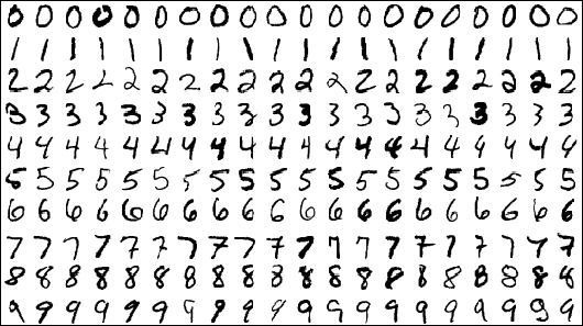
MNIST is a classic image recognition problem, specifically digit recognition. It contains 70,000 28x28 pixel grayscale images of hand-written, labeled images, 60,000 for training and 10,000 for testing. Convolutional Neural Networks (CNN) do really well on MNIST, achieving 99%+ accuracy. The Pytorch distribution includes a 4-layer CNN for solving MNIST. Here I will unpack and go through this example. We use torchvision to avoid downloading and data wrangling the datasets. Finally, instead of calculating performance metrics of the model by hand, I will extract results in a format so we can use SciKit-Learn's rich library of metrics. You can run this on your laptop in a couple of minutes without a GPU, the ipython notebook is up on Github.
The neural network
The definition for the CNN is just a couple of lines, taken from https://github.com/pytorch/examples/blob/master/mnist/main.py:
class CNN(nn.Module):
    def __init__(self):
        super(CNN, self).__init__()
        self.conv1 = nn.Conv2d(1, 20, 5, 1)
        self.conv2 = nn.Conv2d(20, 50, 5, 1)
        self.fc1 = nn.Linear(4*4*50, 500)
        self.fc2 = nn.Linear(500, 10)

    def forward(self, x):
        x = F.relu(self.conv1(x))
        x = F.max_pool2d(x, 2, 2)
        x = F.relu(self.conv2(x))
        x = F.max_pool2d(x, 2, 2)
        x = x.view(-1, 4*4*50)
        x = F.relu(self.fc1(x))
        x = self.fc2(x)
        return F.log_softmax(x, dim=1)
As an exercise, let's make sure we understand what's going on here:
conv1is the first convolutional layer:- the MNIST images are grayscale, so there is just 1 input channel
- this layer computes 20 convolutions, so the output is 20 channels
- each kernel is 5x5
- with a stride of 1
- by default, each kernel has a bias
- 20 x (5 x 5 + 1) = 520 parameters to train
- the input is 28x28 pixels, the ouput is 28 - (5-1) = 24x24 pixels, on 20 channels each
- in
forward(),conv1is applied to the input image, than amax_pool2d()- 2x2 patches are maxpool'd, with a stride of 2, this halves the image
- the input is 24x24 pixels, the output is 12x12 pixels
conv2is the second convolutional layer:- input = 12x12 pixels, 20 channels
- this layer computes 50 convolutions, so the output is 50 channels
- same kernel and stride as the previous layer
- 50 x (20 x 5 x 5 + 1) = 25,050 parameters to train
- the input is 12x12 pixels, the output is 12 - (5-1) = 8x8 pixels, on 50 channels each
- having >1 input and output channels: there is a separate 5x5 kernel for each combination (50x20 kernels), then to get each of the 50 output pixels the 20 convolved are averaged, and the bias is added
- we apply
relu(), this doesn't change dimensionality - another
max_pool2d()follows, cutting image size from 8x8 to 4x4 pixels fc1(for fully connected):- takes the 4 x 4 x 50 = 800 input values and treats is as a big vector
- projects it to a 500 dimensional vector with an Ax+b matrix multiplication
- this is 4 x 4 x 50 x 500 + 500 = 400,500 parameters to train
- then another
relu() fc2- projects down to a 10 dimensional vector
- this is 500 x 10 + 50 = 5,050 parameters to train
- then
log_softmax()to get log-probabilities for each class; regularsoftmax()would output probabilities, but here they arelog()'d, so later we have toexp()to get back the probabilities
Total parameters = 520 + 25,050 + 400,500 + 5,050 = 431,120 floats
Getting data
As mentioned, we use torchvision here:
train_loader = torch.utils.data.DataLoader(
    datasets.MNIST(
        '../data',
       train=True,
       download=True,
       transform=transforms.Compose([
           transforms.ToTensor(),
           transforms.Normalize((0.1307,), (0.3081,))
       ])
    ),
    batch_size=64,
    shuffle=True)
test_loader = torch.utils.data.DataLoader(
    datasets.MNIST(
        '../data',
        train=False,
        transform=transforms.Compose([
           transforms.ToTensor(),
           transforms.Normalize((0.1307,), (0.3081,))
        ])
    ),
    batch_size=1000,
    shuffle=True)
The only trick here is the normalization. The mean and standard deviation passed in is the actual value computed for the dataset, after normalization (subtract and divide) the dataset will be a standard normal N(0,1) distribution. This just helps the training.
Training the model
Training is straightforward. I've modified the code so it returns the losses, so we can plot it later:
def train(model, device, train_loader, optimizer, epoch):
    losses = []
    model.train()
    for batch_idx, (data, target) in enumerate(train_loader):
        data, target = data.to(device), target.to(device)
        optimizer.zero_grad()
        output = model(data)
        loss = F.nll_loss(output, target)
        loss.backward()
        optimizer.step()
        losses.append(loss.item())
        if batch_idx > 0 and batch_idx % 100 == 0:
            print('Train Epoch: {} [{}/{}\t({:.0f}%)]\tLoss: {:.6f}'.format(
                epoch, batch_idx * len(data), len(train_loader.dataset),
                100. * batch_idx / len(train_loader), loss.item()))
    return losses
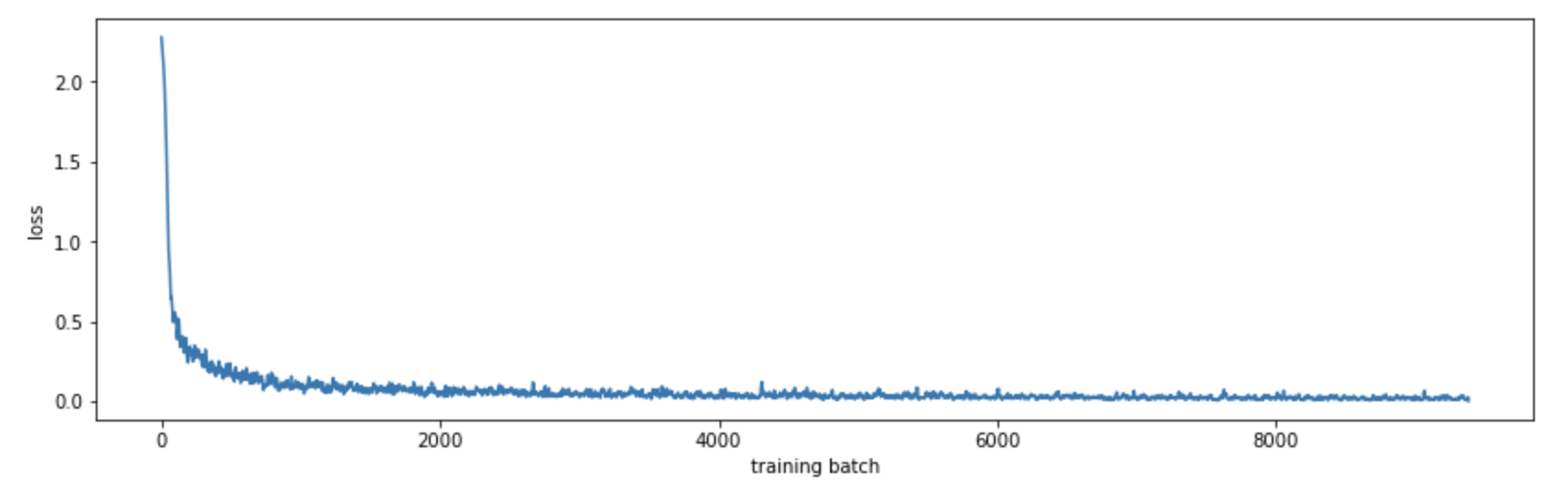
This is a plain vanilla training loop, with nll_loss(). This stands for negative log likelihood (NLL).
NLL essentially transforms the class probability (0 to 1) to run from ∞ to 0, good for a loss function. The combination of outputing log_softmax() and minimizing nll_loss() is mathematically the same as outputing the probabilities and minimizing cross-entropy (how different are two probability distributions, in bits), but with better numerical stability.
Using matplotlib we can see how the model converges:
def mean(li): return sum(li)/len(li)
plt.figure(figsize=(14, 4))
plt.xlabel('training batch')
plt.ylabel('loss')
plt.plot([mean(losses[i:i+10]) for i in range(len(losses))])
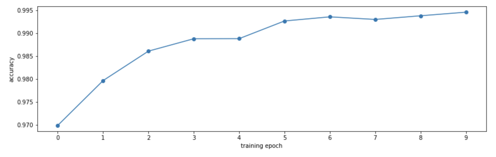
By computing the accuracy on the training set at the end of each epoch, we can see how our model improves:
Evaluating the model
Now we use the test data portion of MNIST, and run the model on it. Most SKL metrics expect 2 of 3 inputs:
- the ground truth labels
- the predicted labels
- the prediction probabilities (for eg. ROC curve)
Now we can use SKL to get various metrics. Because the model performs so well, most of these are not very interesting.
def test_label_predictions(model, device, test_loader):
    model.eval()
    actuals = []
    predictions = []
    with torch.no_grad():
        for data, target in test_loader:
            data, target = data.to(device), target.to(device)
            output = model(data)
            prediction = output.argmax(dim=1, keepdim=True)
            actuals.extend(target.view_as(prediction))
            predictions.extend(prediction)
    return [i.item() for i in actuals], [i.item() for i in predictions]

actuals, predictions = test_label_predictions(model, device, test_loader)
print('Confusion matrix:')
print(confusion_matrix(actuals, predictions))
print('F1 score: %f' % f1_score(actuals, predictions, average='micro'))
print('Accuracy score: %f' % accuracy_score(actuals, predictions))
Outputs:
Confusion matrix:
[[ 973    0    0    0    0    0    4    1    2    0]
 [   0 1130    0    2    0    1    1    1    0    0]
 [   1    1 1024    0    2    0    1    2    1    0]
 [   0    0    0 1005    0    2    0    0    3    0]
 [   0    0    1    0  975    0    1    1    1    3]
 [   2    0    0   11    0  874    2    1    2    0]
 [   0    1    0    0    1    1  955    0    0    0]
 [   0    3    3    1    0    0    0 1019    1    1]
 [   0    0    1    1    0    1    0    0  970    1]
 [   0    2    0    6    7    2    0    4    1  987]]
F1 score: 0.991200
Accuracy score: 0.991200
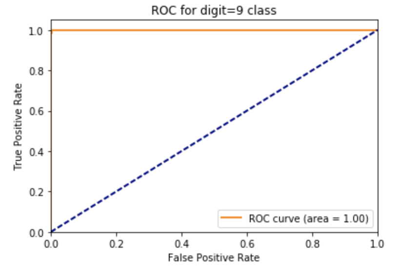
ROC curve for one of the digit classes, with AUC; since the classifier is so good, the ROC curve is the ideal top-right curve, and AUC is 1.0 (again, not very interesting):
def test_class_probabilities(model, device, test_loader, which_class):
    model.eval()
    actuals = []
    probabilities = []
    with torch.no_grad():
        for data, target in test_loader:
            data, target = data.to(device), target.to(device)
            output = model(data)
            prediction = output.argmax(dim=1, keepdim=True)
            actuals.extend(target.view_as(prediction) == which_class)
            probabilities.extend(np.exp(output[:, which_class]))
    return [i.item() for i in actuals], [i.item() for i in probabilities]

which_class = 9
actuals, class_probabilities = test_class_probabilities(model, device, test_loader, which_class)

fpr, tpr, _ = roc_curve(actuals, class_probabilities)
roc_auc = auc(fpr, tpr)
plt.figure()
lw = 2
plt.plot(fpr, tpr, color='darkorange',
         lw=lw, label='ROC curve (area = %0.2f)' % roc_auc)
plt.plot([0, 1], [0, 1], color='navy', lw=lw, linestyle='--')
plt.xlim([0.0, 1.0])
plt.ylim([0.0, 1.05])
plt.xlabel('False Positive Rate')
plt.ylabel('True Positive Rate')
plt.title('ROC for digit=%d class' % which_class)
plt.legend(loc="lower right")
plt.show()
Conclusion
The combination of Pytorch, torchvision and SKL makes it really quick to play around with deep neural network architectures and see how they perform, without writing too much code, while using regular Python to do the debugging. A good next step is to play around with CIFAR data.