SVM with Pytorch

Support Vector Machines are a standard ML model for supervised classification. The basic idea behind a (linear) SVM is to find a separating hyperplane for two categories of points. Additionally, to make the model as generic as possible, SVM tries to make the margin separating the two sets of points as wide as possible. When a linear separator is not enough, SVM can be made non-linear with the kernel trick, but here I will stick to the linear model. All the code is up on Github.

Doing SVM in Pytorch is pretty simple, and we will follow the same recipe as in the Ax=b post. We will use the standard Iris dataset for supervised learning.

Setting up the model: differentiable SVM

In order for Pytorch and autograd to work, we need to formulate the SVM model in a differentiable way. This is pretty straighforward, and has been done before by Tang in this 2013 paper.

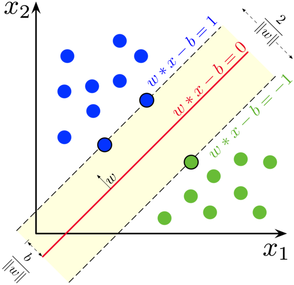
The separating hyperplane is defined by the wx - b = 0 equation, where w is the normal vector and b is a scalar offset. w’s dimendionality is however many features we have. Additionally, we will try to place the plane in such a way that it falls halfway between the two classes, so that, if possible, there are no points behind the wx - b = ±1 lines (see first image). For each training point x, we want wx - b > 1 if x is in the +1 class, wx - b < -1 if x is in the -1 class (we re-label classes to ±1). Calling the labels y, we can multiply both equations to get the same thing: y ( wx - b) > 1, or 1 - y ( wx - b ) < 0.

So our constraint is for these expressions to be less than zero for each training point. If it’s positive, that’s “bad”. If it’s negative, we don’t really care how negative it is. This leads to the loss function: ∑ max[0, 1 - y ( wx - b ) ]. To make it optimizer friendly, we square it: ∑ max[0, 1 - y ( wx - b ) ]².

There is a caveat though. What if the training points overlap? Or, there is just a few points which would cause the separating hyperplane’s margin to be very narrow? As the first picture shows, the width of the margin is 2/|w|, we also want to maximize this, or, minimize |w|/2, so the model generalizes better. So the full loss function is: |w|/2 + C ∑ max[0, 1 - y ( wx - b ) ]². C is an important hyperparameter, it sets the importance of separating all the points and pushing them outside the margin versus getting a wide margin.

Pytorch code

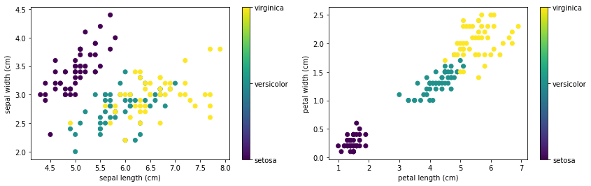
First, let’s get the Iris data. The easiest is to get it from SciKit-Learn, which comes with a bunch of standard datasets. We can use pyplot to visualize Iris’s 4 features and the 3 species:

The code for this is:

from matplotlib import pyplot as plt
from sklearn.datasets import load_iris

def plot(x_index, y_index):
    formatter = plt.FuncFormatter(lambda i, *args: iris.target_names[int(i)])
    plt.scatter(iris.data[:, x_index], iris.data[:, y_index], c=iris.target)
    plt.colorbar(ticks=[0, 1, 2], format=formatter)
    plt.xlabel(iris.feature_names[x_index])
    plt.ylabel(iris.feature_names[y_index])

iris = load_iris()
plt.figure(figsize=(14, 4))
plt.subplot(121)
plot(0, 1)
plt.subplot(122)
plot(2, 3)
plt.show()

For this demonstration, I will just run SVM on the petal length and width (the last two features), and build a setosa vs rest classifier. Constructing the training and test data:

X = [[x[2], x[3]] for x in iris.data]
y = iris.target.copy()
for i in range(len(y)):
    if y[i] == 0: y[i] = 1
    else: y[i] = -1
X_train, X_test, y_train, y_test = train_test_split(X, y, test_size=0.2)

Writing the code is straightforward, it’s the same story as in the Ax=b post. w and b are variables that we want to optimize. For this task we can leave out the first part of the loss function, because an exact solution is possible:

dim = len(X[0])
w = torch.autograd.Variable(torch.rand(dim), requires_grad=True)
b = torch.autograd.Variable(torch.rand(1),   requires_grad=True)

step_size = 1e-3
num_epochs = 5000
minibatch_size = 20

for epoch in range(num_epochs):
    inds = [i for i in range(len(X_train))]
    shuffle(inds)
    for i in range(len(inds)):
        L = max(0, 1 - y_train[inds[i]] * (torch.dot(w, torch.Tensor(X_train[inds[i]])) - b))**2
        if L != 0: # if the loss is zero, Pytorch leaves the variables as a float 0.0, so we can't call backward() on it
            L.backward()
            w.data -= step_size * w.grad.data # step
            b.data -= step_size * b.grad.data # step
            w.grad.data.zero_()
            b.grad.data.zero_()

Let’s print out the w and b values, and evaluate the model:

print('plane equation:  w=', w.detach().numpy(), 'b =', b.detach().numpy()[0])

def accuracy(X, y):
    correct = 0
    for i in range(len(y)):
        y_predicted = int(np.sign((torch.dot(w, torch.Tensor(X[i])) - b).detach().numpy()[0]))
        if y_predicted == y[i]: correct += 1
    return float(correct)/len(y)

print('train accuracy', accuracy(X_train, y_train))
print('test accuracy', accuracy(X_test, y_test))

I get:

plane equation:  w= [-0.8717707 -1.4143362] b = -3.2047558
train accuracy 1.0
test accuracy 1.0

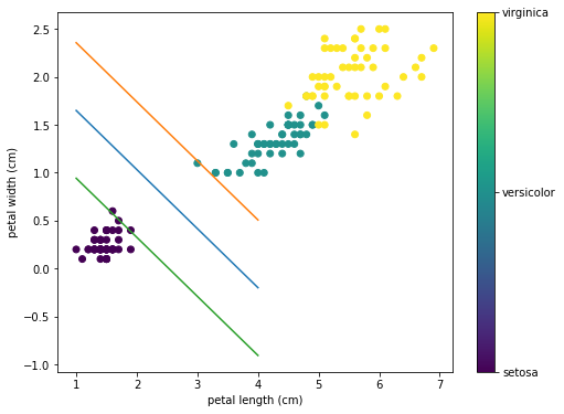
Let’s visualize the solution:

def line_func(x, offset):
    return   -1 * (offset - b.detach().numpy()[0] + w.detach().numpy()[0] * x ) / w.detach().numpy()[1]

x = np.array(range(1, 5))
ym = line_func(x,  0)
yp = line_func(x,  1)
yn = line_func(x, -1)

x_index = 2
y_index = 3
plt.figure(figsize=(8, 6))
formatter = plt.FuncFormatter(lambda i, *args: iris.target_names[int(i)])
plt.scatter(iris.data[:, x_index], iris.data[:, y_index], c=iris.target)
plt.colorbar(ticks=[0, 1, 2], format=formatter)
plt.xlabel(iris.feature_names[x_index])
plt.ylabel(iris.feature_names[y_index])
plt.plot(x, ym)
plt.plot(x, yp)
plt.plot(x, yn)

To get:

This was just a game. There’s no good reason to run SVM on Pytorch, SciKit-Learn has a built-in SVM model that is more robust and scalable and can get this done in less lines of code.