Paper review: A Comparison of Approaches to Advertising Measurement

My summary

Randomized Controlled Trials — also known as A/B testing in the tech industry — are widely regarded as the gold standard of causal inference. What else can a Data Scientist do if RCTs or A/B testing is not possible, and why are alternatives inferior to A/B testing?

The alternative methods are called observational methods, since unlike an A/B test, we do not interfere with the treatment to create a control group. Common observational methods are Exact Matching (EM), Propensity Score Matching (PSM), Stratification and Regression Adjustment (RA). These methods are used if there is:

1. no Control group, everybody was in the Treatment group (eg. "eligible to receive ads on Facebook", or, "received marketing email")
2. the goal, like in RCTs, is to estimate the average treatment effect (eg. signups, checkouts, sales) by comparing exposed and non-exposed treatment users (exposed can mean "viewed ad" or "opened marketing email").

The paper, A Comparison of Approaches to Advertising Measurement: Evidence from Big Field Experiments at Facebook by Gordon and Zettelmeyer shows, using 15 experiments where a RCT was conducted, that common observational methods severely mis-estimate the true treatment lift (as measured by the RCT), often by a factor of 3x or more. This is true, even though Facebook has (i) very large sample sizes, and, (ii) very high quality data (per-user feature vector) about its users which are used in the observational methods. This should be a red flag for Data Scientists working on common marketing measurements using observational methods.

The remainder is direct quotes from the paper with minor grammatical changes. I will highlight parts that I added.

Introduction

Measuring the causal effect of advertising remains challenging for at least two reasons. First, individual-level outcomes are volatile relative to ad spending per customer, such that advertising explains only a small amount of the variation in outcomes. Second, even small amounts of advertising endogeneity (e.g., likely buyers are more likely to be exposed to the ad) can severely bias causal estimates of its effectiveness.

In principle, using large-scale randomized controlled trials (RCTs) to evaluate advertising effectiveness could address these concerns. In practice, however, few online ad campaigns rely on RCTs. Reasons range from the technical difficulty of implementing experimentation in ad-targeting engines to the commonly held view that such experimentation is expensive and often unnecessary relative to alternative methods. Thus, many advertisers and leading ad-measurement companies rely on observational methods to estimate advertising’s causal effect.

We assess empirically whether the variation in data typically available in the advertising industry enables observational methods to recover the causal effects of online advertising. To do so, we use a collection of 15 large-scale advertising campaigns conducted on Facebook as RCTs in 2015. We use this dataset to implement a variety of matching and regression-based methods and compare their results with those obtained from the RCTs.

A fundamental assumption underlying observational models is unconfoundedness: conditional on observables, treatment and (potential) outcomes are independent. Whether this assumption is true depends on the data-generating process, and in particular on the requirement that some random variation exists after conditioning on observables. In our context, (quasi-)random variation in exposure has at least three sources: user-level variation in visits to Facebook, variation in Facebook’s pacing of ad delivery over a campaign’s pre-defined window, and variation due to unrelated advertisers’ bids. All three forces induce randomness in the ad auction outcomes.

An analysis of our 15 Facebook campaigns shows a significant difference in the ad effectiveness obtained from RCTs and from observational approaches based on the data variation at our disposal. Generally, the observational methods overestimate ad effectiveness relative to the RCT, although in some cases, they significantly underestimate effectiveness. The bias can be large: in half of our studies, the estimated percentage increase in purchase outcomes is off by a factor of three across all methods.

These findings represent the first contribution of our paper, namely, to shed light on whether — as is thought in the industry — observational methods using good individual-level data are “good enough” for ad measurement, or whether even good data prove inadequate to yield reliable estimates of advertising effects. Our results support the latter.

Experimental setup

We focus exclusively on campaigns in which the advertiser had a particular “direct response” outcome in mind, for example, to increase sales of a new product. The industry refers to these as “conversion outcomes.” In each study, the advertiser measured conversion outcomes using a piece of Facebook-provided code (“conversion pixel”) embedded on the advertiser’s web pages, indicating whether a user visited that page. Different placement of the pixels can measure different conversion outcomes. A conversion pixel embedded on a checkout-confirmation page, for example, measures a purchase outcome. A conversion pixel on a registration-confirmation page measures a registration outcome, and so on. These pixels allow the advertiser (and Facebook) to record conversions for users in both the control and test group and do not require the user to click on the ad to measure conversion outcomes.

As with most online advertising, each impression is the result of an underlying auction. The auction is a modified version of a second-price auction such that the winning bidder pays only the minimum amount necessary to have won the auction.

An experiment begins with the advertiser deciding which consumers to target with a marketing campaign, such as all women between 18 and 54. These targeting rules define the relevant set of users in the study. Each user is randomly assigned to the control or test group based on a proportion selected by the advertiser, in consultation with Facebook. Control-group members are never exposed to campaign ads during the study; those in the test group are eligible to see the campaign’s ads. Facebook avoids contaminating the control group with exposed users, due to its single-user login feature. Whether test-group users are ultimately exposed to the ads depends on factors such as whether the user accessed Facebook during the study period (we discuss these factors and their implications in the next subsection). Thus, we observe three user groups: control-unexposed, test-unexposed, and test-exposed.

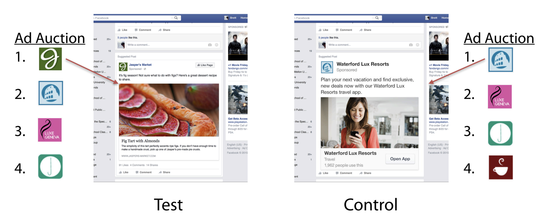
The auction’s second-place ad is served to the control user because that user would have won the auction if the focal ad had not existed.

Sources of endogeneity in this scenario:

• User-induced endogeneity: The first mechanism that drives selection was coined “activity bias” when first identified by Lewis, Rao, and Reiley (2011). In our context, activity bias arises because a user must visit Facebook during the campaign to be exposed. If conversion is a purely digital outcome (e.g., online purchase, registration), exposed users will be more likely to convert merely because they happened to be online during the campaign. For example, a vacationing target-group user may be less likely to visit Facebook and therefore miss the ad campaign. What leads to endogeneity is that the user may also be less likely to engage in any online activities, such as online purchasing. Thus, the conversion rate of the unexposed group provides a biased estimate of the conversion rate of the exposed group had it not been exposed.
• Targeting-induced endogeneity: Assessing ad effectiveness by comparing exposed versus unexposed consumers will overstate the effectiveness of advertising because exposed users were specifically chosen based on their higher conversion rates by the Facebook ML system as it learns as the campaign runs.
• Competition-induced endogeneity: For example, if, during the campaign period, another advertiser bids high on 18-54-year-old women who are also mothers, the likelihood that mothers will not be exposed to the focal campaign is higher.

In the RCT, we address potential selection bias by leveraging the random-assignment mechanism and information on whether a user receives treatment. For the observational models, we discard the randomized control group and address the selection bias by relying solely on the treatment status and observables in the test group.

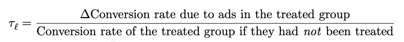
Definition of lift:

Observational methods

Here we present the observational methods we compare with estimates from the RCT. The following thought experiment motivates our analysis. Rather than conducting an RCT, an advertiser (or a third party acting on the advertiser’s behalf) followed customary practice by choosing a target sample and making all users eligible to see the ad. Although all users in the sample are eligible to see the ad, only a subsample is eventually exposed. To estimate the treatment effect, the advertiser compares the outcomes in the exposed group with the outcomes in the unexposed group.

Methods checked in the paper:

• Exact matching (EM):
  • Paper's explanation: Matching is an intuitive method for estimating treatment effects under strong ignorability. To estimate the ATT (Average Treatment Effect on the Treated), matching methods find untreated individuals similar to the treated individuals and use the outcomes from the untreated individuals to impute the missing potential outcomes for the treated individuals. The difference between the actual outcome and the imputed potential outcome is an estimate of the individual-level treatment effect, and averaging over treated individuals yields the ATT. This calculation highlights an appealing aspect of matching methods: they do not assume a particular form for an outcome model.
  • ChatGPT's explanation: This method involves creating pairs of treated and untreated subjects (e.g., those who have and haven't seen an ad) that are identical on all observed covariates, such as demographics or prior purchasing behavior.
  • My explanation: for each exposed user with outcome Y (eg. sales or 0/1 conversion), find M similar unexposed users based on the covariates (ie. the feature vector of the user). Estimate the potential outcome by the average A across the M unexposed users (eg. sales or 0..1 conversion). Compute the difference Y-A. Repeat for all exposed users and average to get ATT.
• Propensity score matching (PSM):
  • ChatGPT's explanation: PSM involves estimating the probability (propensity score) that a subject would be exposed based on observed covariates. Subjects are then matched based on these scores.
  • My explanation: create a [feature-vector → exposure] prediction model where exposure in the training set is a boolean 0/1 for users, the target variable is called the propensity score; the model will return a 0..1 real valued propensity score for each user. For each exposed user with outcome Y, find M similar unexposed users based on the propensity score value (eg. if the exposed user had propensity score 0.765, then find the M unexposed users with propensity score closest to 0.765), and then repeat the same as above to get ATT: Estimate the potential outcome by the average A across the M unexposed users (eg. sales or 0..1 conversion). Compute the difference Y-A. Repeat for all exposed users and average to get ATT.
• Stratification (STRAT):
  • Paper's explanation: The computational burden of matching on the propensity score can be further reduced by stratification on the estimated propensity score (also known as subclassification or blocking). After estimating the propensity score, the sample is divided into strata (or blocks) such that within each stratum, the estimated propensity scores are approximately constant.
  • ChatGPT's explanation: This method involves dividing subjects into subgroups or strata based on their propensity scores and analyzing outcomes within these strata. Often, the propensity scores are divided into quintiles or deciles.
  • My explanation: take the PSM from above, and bucket the propensity scores (eg. into 10 or 100 buckets, depending on sample size N). In each bucket (where we assume users are similar), compute the difference between [average exposed user outcome] and [average unexposed user outcome]. Then take the weighted average of these, weighted by the number of exposed users in each bucket to get the ATT.
• Regression adjustment (RA):
  • Paper's explanation: Whereas exact matching on observables, propensity score matching, and stratification do not rely on an outcome model, another class of methods relies on regression to predict the relationship between treatment and outcomes.
  • ChatGPT's explanation: Regression adjustment involves using regression models to statistically control for differences in covariates between the treated and control groups. The treatment effect is modeled directly, adjusting for covariates that might confound the causal relationship.
  • My explanation: we attempt to construct a linear model Y = C + B * X + ATT * W where Y is the outcome (eg. sales or 0/1 conversion), W=0/1 is whether the user was exposed or not, X is each user's feature vector; C (real), B (vector) and ATT (real) are the result of the fit on doing an OLS on the N rows, one for each user. In this approach, ATT works out to be parameter in the model multiplying W.
• Inverse-probability-weighted regression adjustment (IPWRA)
• Stratification and Regression (STRATREG)

Data

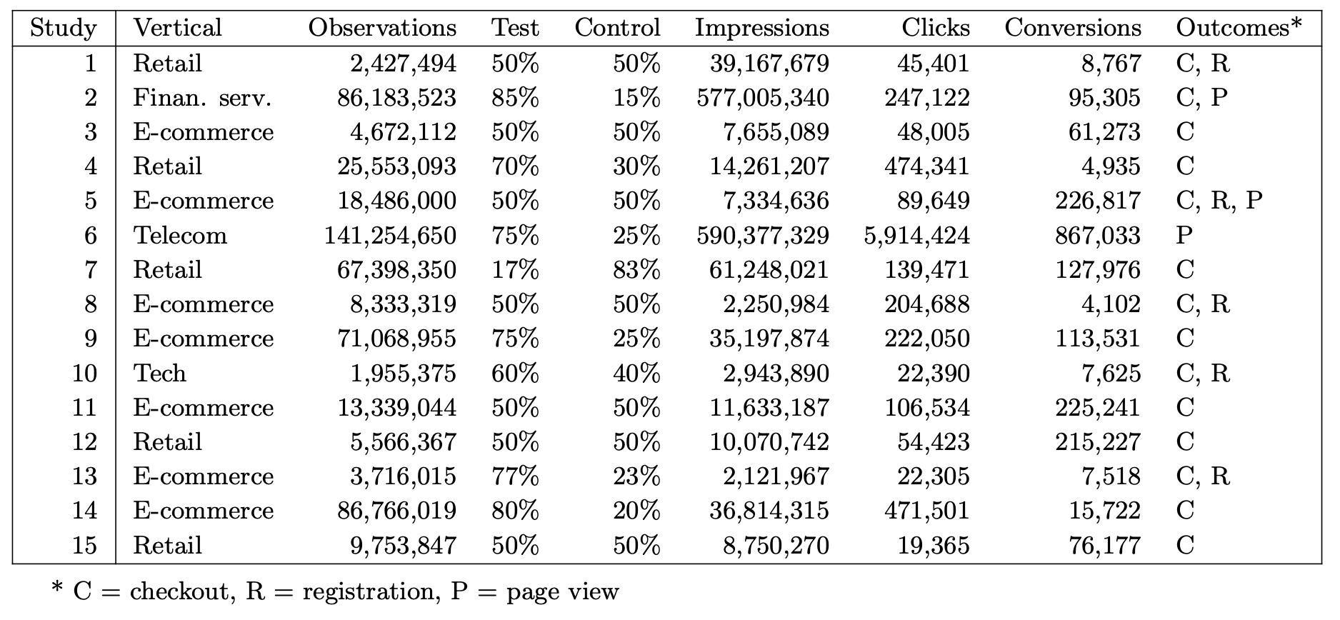
The 15 advertising studies analyzed in this paper were chosen by two of its authors (Gordon and Zettelmeyer) based on criteria to make them suitable for comparing common ad-effectiveness methodologies: conducted after January 2015, when Facebook first made the experimentation platform available to sufficiently large advertisers; minimum sample size of 1 million users; business-relevant conversion tracking in place; no retargeting campaign by the advertiser; and no significant sharing of ads between users. The window during which we obtained studies for this paper was from January to September 2015. Although the sample of studies is not representative of all Facebook advertising (nor is it intended to be), it covers a varied set of verticals (retail, financial services, ecommerce, telecom, and tech), represents a range of sample sizes, and contains a mix of test/control splits. All studies were US-based RCTs, and we restrict attention to users age 18 and older.

Covariates the aka feature vector

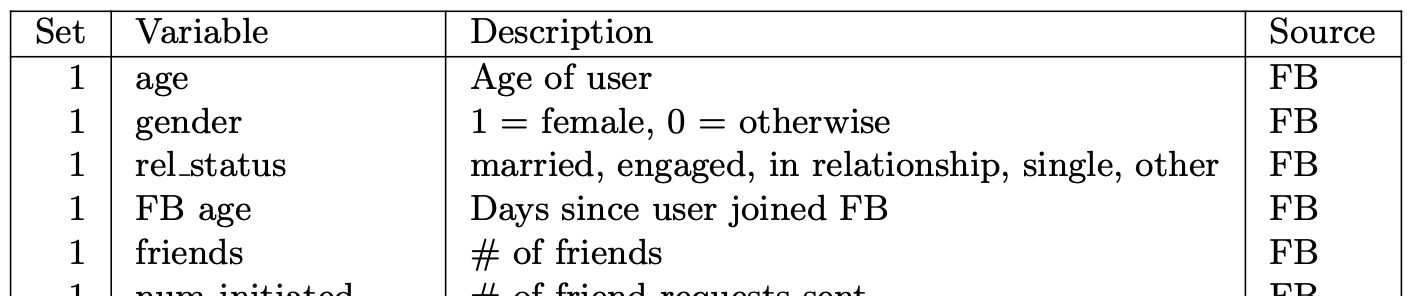
The paper uses the following per-user covariates, in other words the per-user feature vector:

1. FB Variables: common Facebook variables such as age, gender, how long users have been on Facebook, how many Facebook friends they have, their phone OS, and other characteristics.
   
2. Census Variables: In addition to the variables in 1, this specification uses Facebook’s estimate of the user’s zip code to associate with each user nearly 40 variables drawn from the most recent Census and American Communities Surveys (ACS).
   
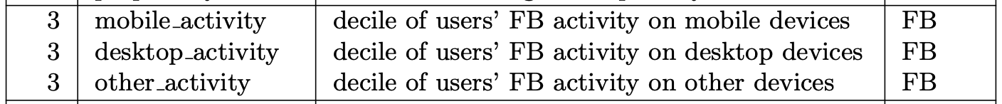
3. User-Activity Variables: In addition to the variables in 2, we incorporate data on a user’s overall level of activity on Facebook. Specifically, for each user and device type (desktop, mobile, or other), the raw activity level is measured as the total number of ad impressions served to that user in the week before the start of any given study.
   
4. Match Score (not important): In addition to the variables in 3, we add a composite metric of Facebook data that summarizes thousands of behavioral variables and is a machine-learning-based metric Facebook uses to construct target audiences similar to consumers an advertiser has identified as desirable.

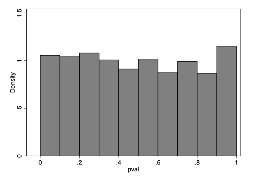
To check whether the randomization of the RCTs was implemented correctly, we compared means across test and control for each study and variable, resulting in 1,251 p-values. Of these, 10% are below 0.10, 4% are below 0.05, and 0.9% are below 0.01. Under the null hypothesis that the means are equal, the resulting p-values from the hypothesis tests should be uniformly distributed on the unit interval. Figure 4 suggests they are and, indeed, a Kolmogorov-Smirnov test fails to reject that the p-values are uniformly distributed on the unit interval (p-value=0.4).

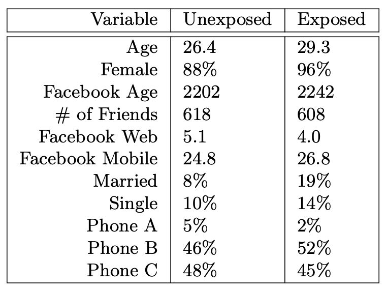
Earlier we noted that we will evaluate observational methods by ignoring our experimental control group and analyzing only consumers in the test group. By doing so, we replicate the situation advertisers face when they rely on observational methods instead of an RCT, namely, to compare exposed to unexposed consumers, all of whom were in the ad’s target group. What selection bias do observational methods have to overcome to replicate the RCT results?

RCT lifts vs observational estimates

How the ATT is computed in the RCTs, to which observational methods are compared, example:

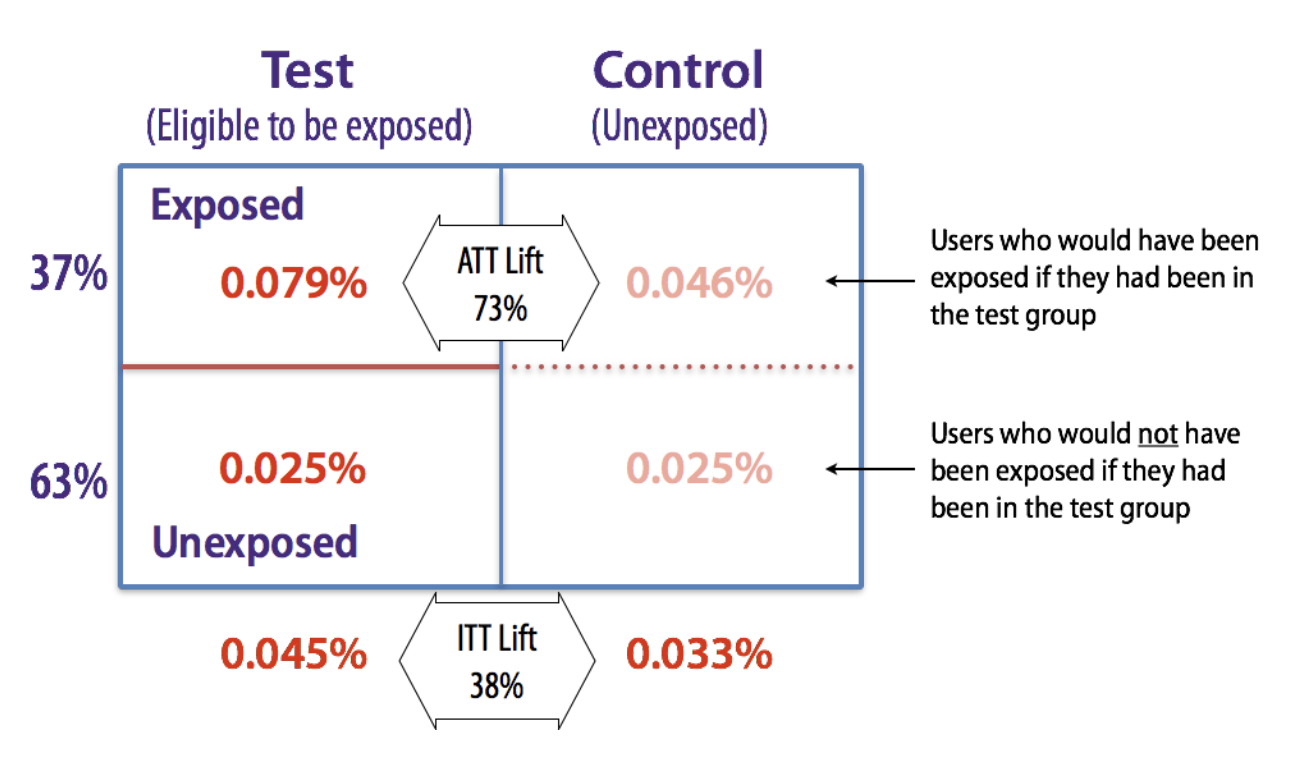
The entries on the x-axis are the observational methods. The dashed line is the actual treatment effect measured using the RCT. The observational methods are estimating that, so ideally should be overlapping, or, close to the dashed line. Some examples:

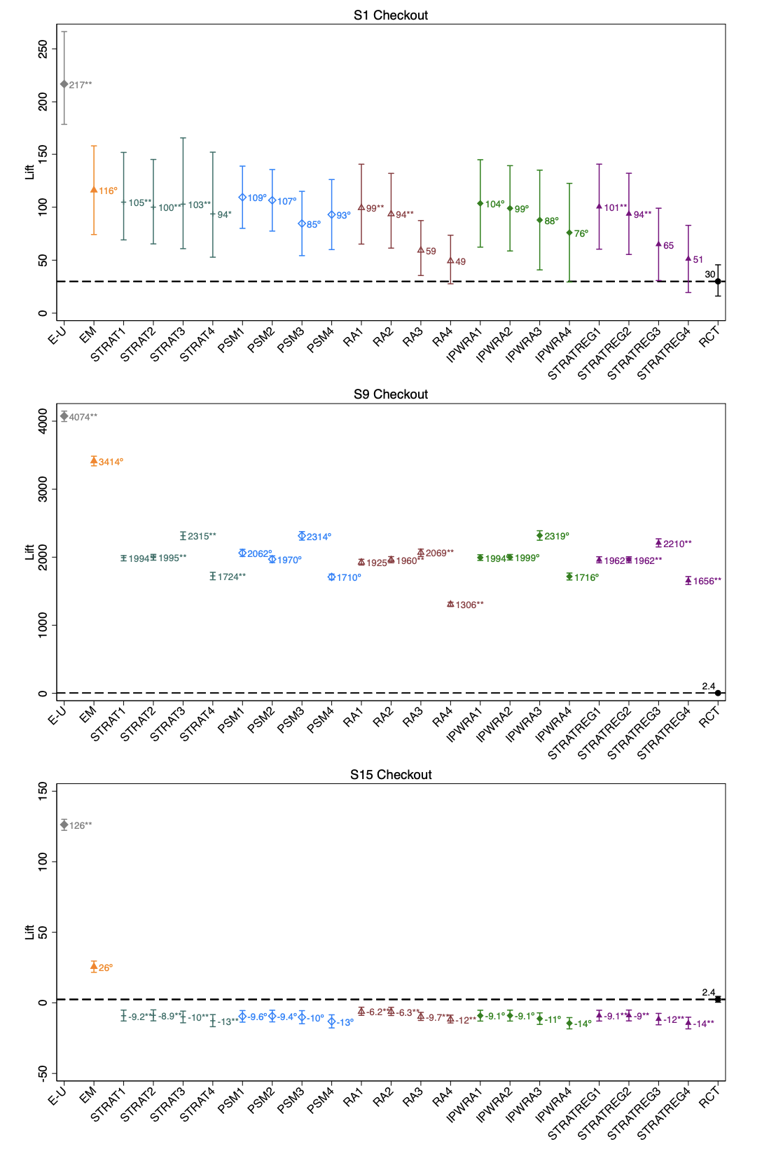
Summary

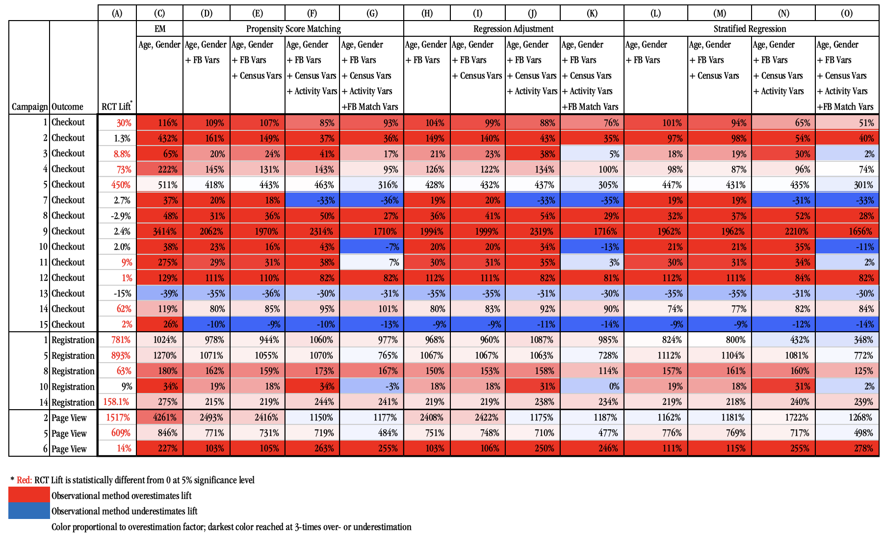
First, the observational methods we study mostly overestimate the RCT lift, although in some cases, they can significantly underestimate RCT lift. Second, the point estimates in seven of the 14 studies with a checkout-conversion outcome are consistently off by more than a factor of three. Third, observational methods do a better job of approximating RCT outcomes for registration and page-view outcomes than for checkouts. We believe the reason is the nature of these outcomes. Because unexposed users (both treatment and control) are relatively unlikely to find a registration or landing page on their own, comparing the exposed group in treatment with a subset of the unexposed group in the treatment group (the comparison all observational methods are based on) yields relatively similar outcomes to comparing the exposed group in treatment with the (always unexposed) control group (the comparison the RCT is based on). Fourth, scanning across approaches, because the exposed-unexposed comparison represents the combined treatment and selection effect—given the nature of selection in this industry—the estimate is always strongly biased up, relative to the RCT lift. Exact matching on gender and age decreases that bias, but it remains significant. Generally, we find that more information helps, but adding census data and activity variables helps less than the Facebook match variable. We do not find that one method consistently dominates: in some cases, a given approach performs better than another for one study but not the other.

Conclusion

In this paper, we have analyzed whether the variation in data typically available in the advertising industry enables observational methods to substitute reliably for randomized experiments in online advertising measurement. We have done so by using a collection of 15 large-scale advertising RCTs conducted at Facebook. We used the outcomes of these studies to reconstruct different sets of observational methods for measuring ad effectiveness, and then compared each of them with the results obtained from the RCT. We find that across the advertising studies, on average, a significant discrepancy exists between the observational approaches and RCTs. The observational methods we analyze mostly overestimate the RCT lift, although in some cases, they significantly underestimate this lift. The bias can be high: in 50% of our studies, the estimated percentage increase in purchase outcomes is off by a factor of three across all methods. With our small number of studies, we could not identify campaign characteristics that are associated with strong biases. We also find that observational methods do a better job of approximating RCT lift for registration and page-view outcomes than for purchases. Finally, we do not find that one method consistently dominates. Instead, a given approach may perform better for one study but not another