A/B testing on social networks

Introduction

In the previous posts on A/B testing we have implicitly assumed independece:

• if $A_1$ and $A_2$ are two units in the A bucket, the choices of $A_1$ and $A_2$ are independent of each other
• the same across A and B

This even went into the math, because the Central Limit Theorem assumes that the random variables added are independent. But the point this post drives home is not going to be about the CLT.

Let’s take the case of post production. An experiment could test whether people are more likely to create a post if the UI element for posting is bigger and more prominent. If this product does not have a sharing/network component, it’s reasonable to make the above 2 independence assumptions. But on a social network the above assumptions do not hold. If the experiment boosts post production, this could lead to their friends seeing more posts in their feed, which in turn could lead to them posting more, which in turn... and so on.

Sticking to the post production example, we can model the effect if we split posting propensity into two parts:

• intrinsic: a random variable which describes how many posts daily a user on the network is likely to create
• network effect: users are more likely to create posts if they see their friends' posts

Let’s assume that group A gets the UI element and it actually boosts their instrinsic post production. Because of the network effect, we expect to:

• measure an increased boost for A (vs just the intrinsic effect), because of A-A “self” interaction (network effect)
• measure an increased boost for B (vs no effect), because of A-B interaction (spillover effect)
• since B is also boosted, A-B interaction also boosts A; everything is boosted, to a different degree

Additionally:

• the effect we measure in A (intrinsic effect plus network effect) will be less than what we get if we release A to 100%, since then the whole network will reinforce
• the network effect depends on the social network: more connections means more reinforcement

The code shown below is up on Github.

Watts–Strogatz random graphs

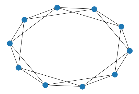
Let’s run some Monte Carlo simulations to see this in action. We will use a random Watts–Strogatz model for the social network, and use the networkx library to generate it for us. The Watts-Strogatz model creates a graph with $n$ nodes, arranged in a ring, with each node connected to the next $k$ nodes in the ring; this initial setup is clustered, and has a high diameter. Then, with probability $p$, each edge is re-connected to a random node on the ring, this causes the diameter of the graph to drop and produces a “small-world graph”, where every node is reachable from every other node in a low number of hops.

Some examples of Watts–Strogatz graphs:

nx.draw(connected_watts_strogatz_graph(n=10, k=4, p=0.0))

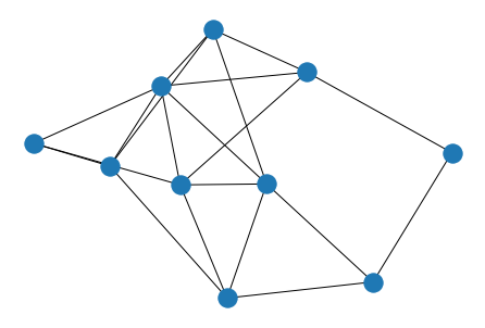
nx.draw(connected_watts_strogatz_graph(n=10, k=4, p=0.5))

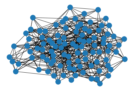
nx.draw(connected_watts_strogatz_graph(n=100, k=10, p=0.5))

For initial exploration, I will use a small graph:

g = connected_watts_strogatz_graph(n=1000, k=50, p=0.1).to_directed()

Post production model

For post production, let’s follow the simple model given above, with two parts:

• intrinsic post production
• network effect: seeing their friends posts causes users to post more, proportionally

In code, we will run the simulation day-to-day, ie. posts from day T will trigger people to post more or day T+1. In this toy model, we will allow non-numeric post production, so people can write eg. 0.1134 posts a day:

def step_posts(g, yesterday_posts=None, intrinsic=0.25, network_effect=0.03):
    today_posts = defaultdict(int)
    # baseline
    for v in g.nodes:
        today_posts[v] = intrinsic * random()
    # network effect
    if yesterday_posts is not None:
        for (v1, v2) in g.edges:
            today_posts[v2] += yesterday_posts[v1] * network_effect * random()
    return today_posts

We can drive it like:

T = 100
posts_series = []
for t in range(T):
    posts = step_posts(g, None if len(posts_series) == 0 else posts_series[-1])
    posts_series.append(posts)

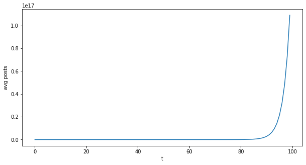
It will take a few days for the network to reach equilibrium:

avg_posts = [np.mean(list(posts.values())) for posts in posts_series]
plt.figure(figsize=(10,5))
plt.xlabel('t')
plt.ylabel('avg posts')
plt.plot(avg_posts)
plt.show()

Prints something like:

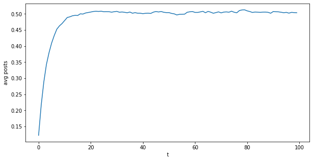
We see that with the parameters used, it converges to 0.5 posts / day on average across the network after about $T_c=20$ steps:

np.mean(avg_posts[20:])

Prints somethings like:

0.5040494951777046

It’s easy to see why. On the first day, each person produces intrinsic * random() posts, where intrinsic = 0.25 and random() is a $U(0, 1)$ uniform random variable, so on average it’s 0.5. So this part is on average $c=0.125$. Then, starting the second day, each person produces $c$ on average, plus for each friend, yesterday_posts[v1] * network_effect * random() additional posts, where network_effect = 0.03, and from the graph each person has 50 friends. So overall this is on average $c * k$, with $k = 50 * 0.03 * 0.5 = 0.75$. Once equilibrium is reached, the following holds: $c_{next} = c + c_{next} * k$. Solving this, $c_{next} = 0.5$.

Note that the intrinsic part averages 0.125, and the network effect adds on another 0.375. In this toy model, 3 out of 4 posts is the result of network effects! This is a good qualitative indication why network effects are so important for engagement.

We can also see that by making the network effect too strong, either by having too many friends or setting network_effect too high, we get exponential growth (in this case, the $c_{next}$ equation yields a nonsensical negative solution). For example, if we double the friend count to 100 (but keep everything else the same):

For the purposes of this discussion, exponential growth is unrealistic. We are assuming there is a base steady-state, and we run an experiment which lifts the steady state by a few percentage points.

Experiments

Let’s do an experiment and see what happens. For this, let's:

• use a bigger graph, with $n=100,000$ nodes, but keep $k=50$
• pick out $N=1,000$ people randomly ("population A"), and boost their intrinsic post production by 5%

Code:

g = connected_watts_strogatz_graph(n=100*1000, k=50, p=0.1).to_directed()
N = 1000
population_A = set(sample(g.nodes, N))
effect_size = 0.05

def step_posts(g, yesterday_posts=None, intrinsic=0.25, network_effect=0.03):
    today_posts = defaultdict(int)
    # baseline
    for v in g.nodes:
        if v in population_A:
            # experiment
            today_posts[v] = intrinsic * random() * (1 + effect_size)
        else:
            today_posts[v] = intrinsic * random()
    # network effect
    if yesterday_posts is not None:
        for (v1, v2) in g.edges:
            today_posts[v2] += yesterday_posts[v1] * network_effect * random()
    return today_posts

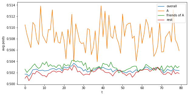
Looking at the converged part of the timeline, this is what we get for (i) overall post production (ii) just A (iii) friends of A and (iv) rest:

Combining all the days, we can get better statistics:

base = 0.5
def lift(a): return ((np.mean(a)/base-1)*100)
print("A lift: %.3f%%" % lift(avg_posts_A))
print("Friends of A lift: %.3f%%" % lift(avg_posts_A_friends))
print("Rest lift: %.3f%%" % lift(avg_posts_rest))
print("Overall lift: %.3f%%" % lift(avg_posts_all))

So compared to the base of 0.5 (no experiment), we measure:

A lift:            1.702%
Friends of A lift: 0.605%
Rest lift:         0.411%
Overall lift:      0.501%

These results are very interesting:

• intrinsic production dampened by the network effect: we underestimate the true intrinsic effect (1.7% vs 5%), because A’s non-A friends don’t have the feature, so As don’t get the boost “back” through these edges
• spillover effect: we measure a lift due to the network effect for friends of A, and further down the network, depending on the distance from As
• if we release this feature to the entire network, average post production would be $ (1 + 0.05) \times 0.25 \times 0.5 / (1 - 50 \times 0.5 \times 0.03) = 0.525$, or a 5% lift compared to the base of 0.5, as expected
• the overall lift is higher than the “rest” because A is pulling it up
• the last 2 lifts (rest and overall) can be made arbitrarily small by increasing the overall size $n$ of the network while keeping the experimental group size $N$ fixed

Intrinsic production dampened by the network effect is a function of the relative strength of the network effect. In this simulation, we set the parameters so that the network effect is very strong, and boosts average post production from 0.125 to 0.5, by 4x! If the network effect were weaker, the experimental dampening would also be weaker, and the same for the spillover effect.

We can see this in action by repeating the experiment with network_effect = 0.01, so a 3x weaker network effect. In this case, the base value works out to 0.1666 (no experiment), so the network effect only boosts post production by 1.666/1.25=1.3x. In the experiment, compared to the base, we measure (with +5% post production for the $N=1000$ population A):

A lift:            3.777%
Friends of A lift: 0.070%
Rest lift:         0.032%
Overall lift:      0.085%

This confirms the above: if the network effect is weaker, the measured lift in the experimental group is closer to the effect size because network effect dampening is lower (3.77% vs 1.70%), while the spillover effect is lower (0.07% vs 0.60%). We can achieve the same effect of making the network effect smaller by decreasing the edge count of the graph, ie. we would get the same result by using a $k=50/3$ Watts–Strogatz graph instead of a $k=50$ one.

Another interesting experiment is if we pick a highly clustered population for the experiment group A. We can achieve this by:

population_A = set(list(g.nodes)[:N])   # set(sample(g.nodes, N)) <- original sampling

First, let’s make sure that this way of picking out $N=1,000$ is in fact more highly clustered than properly sampling. In the original setup, we expect each A to have on average N/n = 1% of neighbours that are also in A, whereas by picking out N subsequent nodes, since only $p=0.1$ portion of edges were re-arranged in the Watts-Strogatz process, we expect this ratio to be significantly higher:

def ratio_AA_friendship(g, population_A):
    num_AA_edges = sum([(v1 in population_A and v2 in population_A) for (v1, v2) in g.edges])
    num_A_edges = sum([(v1 in population_A) for (v1, _) in g.edges])
    return num_AA_edges / num_A_edges

print('%.2f'% ratio_AA_friendship(g, set(sample(g.nodes, N))))
print('%.2f'% ratio_AA_friendship(g, set(list(g.nodes)[:N])))

Prints something like:

0.01
0.89

With proper random sampling, the ratio is indeed 1%, whereas in the highly clustered case 89% of A’s friends are also As. So in this setup, we expect the measured A lift to be much closer to the true lift of 5% (using the original network_effect = 0.03). Running the simulation with this clustered A population, we get:

A lift:            4.307%
Friends of A lift: 0.579%
Rest lift:         0.460%
Overall lift:      0.508%

The result is as expected: the measured lift is much closer to the true lift than with a true random sampled A population (4.3% is much closer to 5% than 1.7% is). It’s interesting that the friends of A lift is not much different (0.58% vs 0.60%). If A is more clustered, the set of non-A friends will be smaller (because there’s less edges going to non-As), but each of them on average (at least in the high $n$ limit) still has the same number of A friends, so the A boost they get will be similar.

Conclusion

When there are no network effects, or they are weak, a regular A/B test with one of the tests discussed in earlier posts works fine. But if there are strong network effects, these have to be taken into account when estimating lift and p-values. In real life there are a lot more nuances to take into account, both related to the network effects and otherwise (eg. cannibalizing photo posts when testing video post lift).