Conditional Probabilities and Simpson's Paradox

Introduction

Recently I was reading the excellent book Patterns, Predictions and Actions, which mentions the Simpson's paradox on page 176, in the chapter on Causality. I've encountered Simpson's paradox before, but like any good paradox, I have to take a step back, think things through and convince myself I understand what's going on each time. This time I decided to write it down to make it more sticky!

University admissions

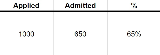
Simpson's paradox is usually explained using the toy example of University admissions and gender bias. Suppose there is a University, and there are $N=1000$ applicants, 650 are admitted, leading to an admission rate of 65%. So far so good.

Now, suppose that of the $N=1000$ applicants, half are male and half are female. Out of 500 males, 400 were admitted, so the admission rate was 80%. Out of 500 females, 250 were admitted, so the admission rate was 50%. Note that the numbers add, up, $ 400+250=650 $ total admissions.

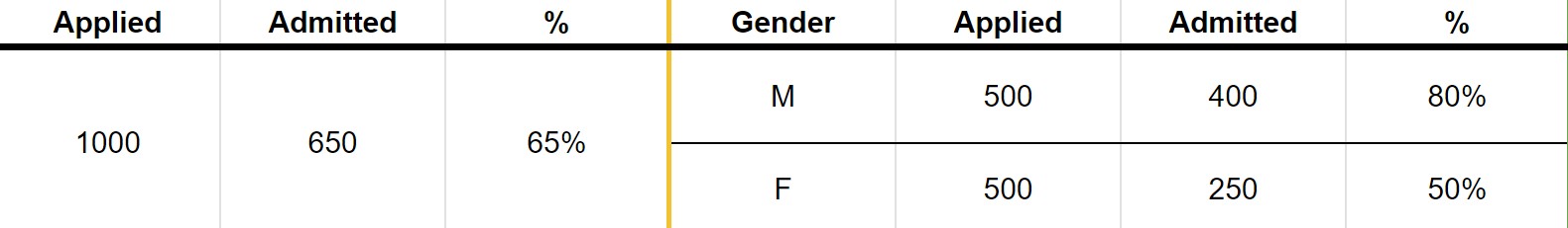
The differing rates of admission may lead us to think that there is gender bias, and the University is discriminating against females. A χ² hypothesis test tells us that the difference in acceptance rates in the two branches (male and female) are statistically significant at $ p < 0.001 $.

Can we stop here? Let's dig deeper: when students apply for University, they actually apply to department, and it's the department that accepts or rejects them. For simplicity, let's assume that each student only applies to one department, and that there are 2 departments, A and B. Simpson's paradox can now manifest itself.

No discrimination

First, let's look at an example where, once we look at the per-deparment admissions, we can convince ourselves that there is no discrimination:

Here, department A has a 90% acceptance rate across both males and females, and department B has a 40% acceptance rate across both males and females. Clearly, there is no discrimination at acceptance. The differing acceptance rate at the male-female level is because 400 out of 500 females apply to the more competitive B department, but only 100 out of 500 males do so.

Reversed discrimination

By playing around with the numbers, it's easy to create a situation where the perceived discrimination is reversed (changed numbers in red):

In this toy example, at the male-female level males have a higher acceptance rate (70% vs 50%), but at the department level, females actually have higher acceptance rates (90% vs 80% for department A and 40% vs 30% for department B). The root cause is the same: even though females are actually more successful at the department level, more of them apply to the more competitive department, leading to lower overall acceptance rates. Note that the same way if would have been erroneous to conclude discrimination without understanding the admission process and seeing the per-department data, it may equally be erroneous to conclude that there is reverse discrimination at the department level; perhaps there are other factors, more depth at play that lead to this outcome.

Same rates

For completeness, we can of course also have a situation where the per-department acceptance rate happen to match the University level (changed numbers in red):

Conditional probability

The "root cause" of these scenarion is simple: in general, there is no relationship between $ P(X=x) $ and $ P(X=x|Y=y) $. All three of the relations equals, less-than or greater-than are possible, and the same goes for $P(X=x|Y=y)$ and $P(X=x|Y=y,Z=z)$.

In our example, if we define $A$ as admission, $G$ as Gender and $D$ as deparment, and treat admission rate as a probability, than $P(A=a), P(A=a|G=g)$ and $P(A=a|G=g,D=d)$, as the above examples show, can be in any relation with each other.

Observation, not experiment

A novice Data Scientists may get confused and wonder: if an run an A/B test and detect a statistically significant difference, how do I know there is no Simpson's paradox lurking in the background? If you're a Data Scientist, I recommend you pause and try to answer this for yourself!

First of all, the example we described above was observational: we didn't interact with the system (applicants or departments), we simply observed the outcomes. In an A/B test (Randomized Controlled Experiment), we conduct an experiment, which means we interact with the system:

1. We randomly split our population into Treatment (A) and Control (B)
2. We treat units in Treatment, but leave units in Control alone.

The whole point of an A/B test is that with enough sample size $N$ (or good stratification), the two populations in A and B will be:

1. the same
2. the same as the overall population

This means that Simpson's paradox cannot occur (other than by variation, which can be limited by the afore-mentioned methods), because sub-population sizes will be the same! Ie. M and F were to branches of an A/B test (which they are not), than the number of people applying to the two departments would be roughly the same; that's the whole point of randomization!

Conclusion

One important conclusion is that a statistical significance test didn't help here; all it told us that the two are in fact different (the normal distributions of the means are far away), but in general a statistical test does not tell us about the reasons two means are different. It is an error of (statistical and logical) reasoning to say "I think X and Y are different because of Z", then use a statistical significance test to establish that "X and Y are indeed different", and then conclude, "therefore Z".

Another suspision is that Simpson's Paradox is more likely to occur if the rates we see reinforce a social construct or stereotype. For example, it's common today to look for gender bias and discrimiation, so it's easier to draw erroneous conclusions around this topic. In other words, we can construct an identical toy example with different words, and the result is less surprising: Ants of colony A have lower lifespans than ants of colony B, even though warrior and harvester ants of both colonies have equal survival probabilities, because colony A has more warrior ants, which have lower lifespans than harvester ants. This, to me is less surprising and less counterintuitive than the original University toy example with genders.