Entropy in Data Science
Marton Trencseni - Sun 24 October 2021 - Math
Introduction
I first wrote about entropy in What's the entropy of a fair coin toss? followed by Cross entropy, joint entropy, conditional entropy and relative entropy, which explained these different entropy-related concepts. Now I will discuss 4 uses of entropy in Data Science:
- Cross entropy as a loss function for training neural network classifiers
- Entropy as a splitting criterion for building decision trees
- Entropy for evaluating clustering algorithms
- Entropy for understanding relationships in tabular data
Cross entropy as a loss function
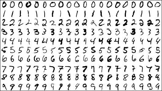
When building a supervised neural network classifier, cross entropy or relative entropy (usually called Kullback–Leibler divergence in Deep Learning frameworks) are common loss functions. For example, suppose we're building an MNIST digit classifier, so there are 10 output classes, corresponding to digits 0..9. Since there are 10 classes, the neural network has 10 outputs. When the network is being trained, for each input image we know the actual digits it's showing, which we encode in a vector like $v_{actual}=[0,0,..,1]$. Since the last number is 1, this is a digit 9. Then we run the input image through the neural network, and read out the outputs for the 10 classes, which may look like $v_{predicted}=[0.1, 0, 0, ... 0, 0.1, 0.8]$. To make sure the output probabilities some to 1, we always put a softmax layer as the last layer of the network. So in this case, the cross entropy loss is $H(p=actual, q=predicted) = -\sum_i p_i log [ q_i ] = - log [ 0.8 ] $. In this expression the only $p_i$ that's non-zero is the one for the actual class, and for that $p_i = 1$, so cross entropy loss really only contains that one term. Note that during actual training, cross entropy loss is computed (summed) for an entire minibatch, ie. multiple training points.
It would be tempting to say that cross entropy loss doesn't care what probabilities the model assigns to the incorrect classes, but this is misleading. As mentioned before, to get the probabilities of the output layer to sum to 1, the last layer is always a softmax, and each of the output probabilities depends on all the outputs of the previous layer. In the MNIST case, we have 10 outputs $z_i$, which are then softmax'd like $q_i = \frac{e^{z_i}}{\sum_j e^{z_j}}$, the divident contains all $z_i$s, so $q_i = q_i(z_0 ... z_9)$.
What's the difference between cross entropy and relative entropy as a loss function? In neural networks, the training method is usually some form of gradient descent, which means that the loss function is differentiated by the weights of the neural network. Per the previous article, relative entropy and cross entropy are related like $ D_{KL}(actual | predicted) = H(actual, predicted) - H(actual) $. Here, $H(actual)$ is a constant with respect to the network weights [but it changes for each mini-batch], so it's derivative wrt to the network weights is 0. Because of this, although the two loss values are different, their derivatives wrt network weights are identical ( $ \frac{\partial D_{KL}(actual | predicted)}{\partial w_i} = \frac{\partial H(actual, predicted)}{\partial w_i} $ because $ \frac{\partial H(actual)}{\partial w_i} = 0$ ), so their usage is equivalent, since the computed gradients propagated back into the network will be exactly the same!
See the Bytepawn article Solving MNIST with Pytorch and SKL for an example Pytorch deep neural network classifier using cross entropy.
Entropy in decision tree classifiers
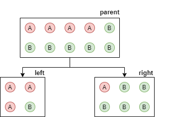
When building a decision tree, the algorithm starts with just one root nodes which contains all samples. Then, at each step, leaf nodes are split into 2 child nodes until a stopping condition is met. Given a set $S$ of samples in the current node to be split, what is the criterion to divide it into two children $S_L$ and $S_R$? If we look at Scikit Learn's DecisionTreeClassifier, the first parameter is called criterion and can either be gini or entropy. Let's look at entropy: in this case, the algorithm will try to split to maximize Information Gain, which is defined as $I = H_{parent} - H_{children}$. Here $H_{parent}$ is the entropy of all samples in the parent node, where probability is just the frequency. So if the parent node contains 4 samples for class A and 6 samples for class B, then $H_{parent} = H([4,6]) = -\frac{4}{10}log\frac{4}{10} - \frac{6}{10}log\frac{6}{10} = 0.97$ bits. Suppose the algorithm is evaluating a split where the left side contains $[A,B]=[3, 1]$ samples and the right side contains $[A,B]=[1, 5]$ samples. So $H_{left} = H([3, 1]) = -\frac{3}{4}log\frac{3}{4} - \frac{1}{4}log\frac{1}{4} = 0.81$ bits. For the right side, $H_{right} = H([1, 5]) = -\frac{1}{6}log\frac{1}{6} - \frac{5}{6}log\frac{5}{6} = 0.65$ bits. Then, $H_{children}$ is sum of these two entropies, weighted by sample size: $H_{children} = \frac{4}{10} H_{left} + \frac{6}{10} H_{right} = 0.71$ bits. So the information gain is $I = H_{parent} - H_{children} = 0.26$ bits. The algorithm looks at multiple possible splits, and selects the one with the highest information gain. Note that if it finds a way to put all As into the left node and all Bs into right node (or vica versa), then the child entropies will be 0, this is the maximum achievable $I_{max}=H_{parent}$, the best possible outcome of the split. Note that Gini impurity is also related to the concept of entropy.
Entropy in clustering
Suppose we want to evaluate some unsupervised clustering algorithms, or the same algorithm with different feature vectors. We have some labeled data, so we can compare the cluster classification to the real classes. So we have for each sample point $i$ a feature vector $x_i$, actual class $A_i$ and the clustering algorithm's cluster identity ie. the modeled class $M_i$. Note that the $M_i$s will not be labeled, since a clustering algorithm just says that a subset of points belong to a cluster, but it doesn't know what that cluster is, there is no name given to it. The $A_i$s are usually labeled, like car, boat, airplane. Because the $A_i$s and $M_i$s are different, cross entropy and relative entropy don't make sense here, since there it's assumed that the two random variables take on the same values.
One approach is to take each cluster (so set of points where $M_i$ is the same), and calculate the entropy using the $A_i$s. We want this to be low, since that corresponds to a cluster with lots of points with the same actual class. Do this for each cluster, and then take the weighted sum of per-cluster entropies. What I described is just the conditional entropy $H(A|M)$! The downside of using conditional entropy is that it can be gamed by creating a lot of little clusters; in the worst case, each point is its own cluster, and all per-cluster entropies are 0. This is best controlled by limiting the number of clusters the clustering algorithm is allowed to create to the number of actual classes.
A better alternative is to use mutual information $I(A, C)$, which will be zero if $A$ and $M$ are completely independent (worst case), and maximal if $A$ and $M$ completely detemine each other, ie. if there are an exactly equal number of classes, and knowing a modeled class $M_i$ always corresponds to the same $A_i$, and vica versa. For more, see this article.
The implementation of the above clustering metrics are straightforward in Python. To demonstrate, let's use the standard Iris flower dataset, which has 4 float numbers describing the length and the width of the sepals and petals in centimeters, and a label for the type of iris (setosa, versicolor, virginica). Let's use k-means clustering from Scikit learn and have it return 3 clusters. Then, let's compute both the conditional entropy and information gain between the modeled and actual classes. Let's see what happens if we run the clustering with just 1, 2, 3 or all 4 of the available feature vector elements:
from math import log
from sklearn import datasets
from sklearn.cluster import KMeans
from collections import defaultdict, Counter

def iris_clusters(use_columns=None):
    iris = datasets.load_iris()
    model = KMeans(n_clusters=len(iris.target_names))
    if use_columns is None:
        data = iris.data
    else:
        data = iris.data[:, use_columns]
    model.fit(data)
    return iris.target, model.predict(data)

def entropy(frequencies, base=2):
    return -1 * sum([f/sum(frequencies) * log(f/sum(frequencies), base) for f in frequencies])

def conditional_entropy(y, x, base=2): # computes H(Y|X)
    clusters = defaultdict(lambda: [])
    for yy, xx in zip(y, x):
        clusters[xx].append(yy)
    return sum([len(cluster)/len(x) * entropy(Counter(cluster).values(), base) for cluster in clusters.values()])

def information_gain(p, q, base=2):
    return     entropy(Counter(p).values(), base) - conditional_entropy(p, q, base)
    # same as  entropy(Counter(q).values()) - conditional_entropy(q, p)

for use_columns in [[0], [0, 1], [0, 1, 2], [0, 1, 2, 3]]:
    actuals, modeled = iris_clusters(use_columns)
    print('Using %d columns in feature vector, conditional entropy = %.2f bits, information gain = %.2f bits' %
          (len(use_columns), conditional_entropy(actuals, modeled), information_gain(actuals, modeled)))
Prints:
Using 1 columns in feature vector, conditional entropy = 0.99 bits, information gain = 0.60 bits
Using 2 columns in feature vector, conditional entropy = 0.56 bits, information gain = 1.02 bits
Using 3 columns in feature vector, conditional entropy = 0.44 bits, information gain = 1.14 bits
Using 4 columns in feature vector, conditional entropy = 0.39 bits, information gain = 1.19 bits
The result is as expected, allowing the clustering algorithm to see more of the feature vector yields lower relative entropy (better) and higher informationg gain (better).
Entropy for understanding columnar data
We can use entropy to see how much information is contained in a column. For example, suppose we have a table users, which has a column country. We know that most of our users are located in our home country, but there may be others. We can compute the per-column entropy with a bit of SQL:
WITH
counts AS
(
    SELECT
        country,
        COUNT(*) AS cnt
    FROM
        users
    WHERE
        country IS NOT NULL
    GROUP BY GROUPING SETS
        ((), (country))
    -- there will be one row with country = NULL, corresponding to the overall counts
    -- the rest of the rows are the country-wise counts
),
probs AS
(
    SELECT
        g.country,
        CAST(g.cnt AS FLOAT) / a.cnt AS p
    FROM
        (SELECT * FROM counts WHERE country IS NOT NULL) g
    CROSS JOIN
        (SELECT * FROM counts WHERE country IS NULL) a
)
SELECT
    -1 * SUM(p * log(2, p)) AS entropy_bits
FROM
    probs
This snippet can be extended to handle more columns, the simplest method is to concatenate columns like '(' || col1 || ',' || col2 || ... ')'. Note that if entropy_bits is 0, it means all values in the column are the same. Interestingly, the entropy (in bits) we compute is also the number of bits a database engine would need to efficiently encode these values in a row-wise manner.
We can also check if another column contains additional information. Suppose there is another column in users called locale, which is the language locale of their browser, like en_us or fr_fr. For this we can use conditional entropy H(locale|country):
WITH
counts AS
(
    SELECT
        country,
        locale,
        COUNT(*) AS cnt
    FROM
        users
    WHERE
        country IS NOT NULL AND locale IS NOT NULL
    GROUP BY GROUPING SETS
        ((), (country), (country, locale))
),
marginal_probs AS
(
    SELECT
        g.country,
        CAST(g.cnt AS FLOAT) / a.cnt AS p
    FROM
        (SELECT * FROM counts WHERE country IS NOT NULL AND locale IS NULL) g
    CROSS JOIN
        (SELECT * FROM counts WHERE country IS NULL AND locale IS NULL) a
),
joint_probs AS
(
    SELECT
        g.country,
        g.locale,
        CAST(g.cnt AS FLOAT) / a.cnt AS p
    FROM
        (SELECT * FROM counts WHERE country IS NOT NULL AND locale IS NOT NULL) g
    CROSS JOIN
        (SELECT * FROM counts WHERE country IS NULL AND locale IS NULL) a
)
SELECT
    -1 * SUM(xy.p * log(2, xy.p/x.p) AS entropy_bits
FROM
    marginal_probs AS x
INNER JOIN
    joint_probs AS xy
USING
    (country)
For example, if country -> locale is a deterministic mapping, ie. USA always maps to en_us, then conditional entropy will be 0. As in earlier examples, information gain also makes sense for tabular data.
Conclusion
The above examples show that entropy is a common and useful concept in Data Science. I plan to write a follow-up article about interesting examples of entropy in Physics.