Probabilistic spin glass - Part I

Introduction

In the previous articles I talked about entropy, and as an example of entropy in Physics, I derived the Sackur-Tetrode entropy of a monatomic ideal glass. Here I will discuss what I call probabilistic spin glass, a simple mathematical model of magnetized matter with short range interactions. In this article I introduce the concept and run some Monte Carlo simulations to get a feel for the model, and use entropy to characterize its order-disorder transition. The code is up on Github.

Probabilistic spin glass

Let's take an $N \times N$ sized spin system, ie. each cell has two states, ↑ and ↓, or 0 and 1. If each spin is indepdendent of its neighbours, then the whole system is just a list of indepdendent random variables, the geometry doesn't matter. To make it interesting, let's make the spins dependent on the neighbours: for spin $s$ and neighbour $n$: $P(s=↑ | n=↑) = P(s=↓ | n=↓) = p$. So the spins align with probability $p$ and are opposite with probability $1-p$.

Monte Carlo simulations

Let's take the above and run Monte Carlo simulations to see what happens as we vary $p$. We will take an array of size $N \times N$ and start filling out the spins according to the probabilities above. First we have to introduce an additional probability $p_0$, which is the probability of the first (let's say top left) spin being ↑. Once we set the first spin, we can set the rest of the spins in the first row. Once we get to the second row, we run into a difficulty. The spins above it have already been set, so these spins have 2 set neighbours. We need to compute the conditional probability $P(s=↑ | n_1=., n_2=.)$ given 2 neighbours $n_1$ and $n_2$ in a way that is consistent with the basic definition of $p$. Using Bayes' theorem, for the specific case of $P(s=↑ | n_1=↑, n_2=↑)$:

$P(s=↑ | n_1=↑, n_2=↑) = \frac{P(s=↑, n_1=↑, n_2=↑)}{P(s=↑, n_1=↑, n_2=↑) + P(s=↓, n_1=↑, n_2=↑)} $

The joint triplet probabilities are easy to compute, we can think of setting $s$ first with probability $p_0$, and then the left and right neighbour with probability $p$:

$P(s=↑, n_1=↑, n_2=↑) = p_0 p^2$

Expressed as Python code calculate_conditional_probs_for_1() returns the conditional probabilities for $P(s=↑, n_1=., n_2=.)$:

def calculate_conditional_probs_for_1(p0, p):
    q = 1 - p
    joint_probs = {
        '000': p0 * p * p,
        '111': p0 * p * p,
        '010': p0 * q * q,
        '101': p0 * q * q,
        '110': p0 * p * q,
        '011': p0 * p * q,
        '001': p0 * p * q,
        '100': p0 * p * q,
    }
    return {
        '00': joint_probs['010']/(joint_probs['010']+joint_probs['000']),
        '01': joint_probs['011']/(joint_probs['011']+joint_probs['001']),
        '10': joint_probs['110']/(joint_probs['110']+joint_probs['100']),
        '11': joint_probs['111']/(joint_probs['111']+joint_probs['101']),
    }

The rest of the system:

def make_unconditional_set(p0):
    return lambda: random() < p0

def make_conditional_set_one_neighbour(p):
    return lambda n: (n) if (random() < p) else (1 - n)

def make_conditional_set_two_neighbours(p0, p):
    conditional_probs_for_1 = calculate_conditional_probs_for_1(p0, p)
    return lambda n1, n2: random() < conditional_probs_for_1[str(int(n1))+str(int(n2))]

def create_grid(rows, cols, p0, p):
    unconditional_set = make_unconditional_set(p0)
    conditional_set_one_neighbour = make_conditional_set_one_neighbour(p)
    conditional_set_two_neighbours = make_conditional_set_two_neighbours(p0, p)
    grid = np.zeros([rows, cols], dtype=np.bool)    
    # first element
    grid[0, 0] = unconditional_set()
    # first row
    for j in range(1, cols):
        grid[0, j] = conditional_set_one_neighbour(grid[0, j-1])
    # remaining rows
    for i in range(1, rows):
        grid[i, 0] = conditional_set_one_neighbour(grid[i-1, 0])
        for j in range(1, cols):
            grid[i, j] = conditional_set_two_neighbours(grid[i-1, j], grid[i, j-1])
    return grid

def show(grid):
    plt.imshow(grid, cmap='hot', interpolation='nearest')
    plt.show()

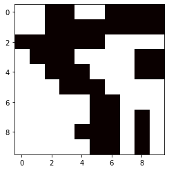
Let's run it with $p_0=0.5$ and $p=0.7$ and see a realization:

show(create_grid(rows=10, cols=10, p0=0.5, p=0.7))

Validation

First, let's make sure the math and logic is correct. Let's simulate a large $100 \times 100$ spin glass with the above rules, then count all pairs, and make sure that the original conditional probability holds:

# consistency check
num_simulations = 100
rows, cols, p0, p = 100, 100, 0.5, 0.70
same, total = 0, 0
for _ in range(num_simulations):
    grid = create_grid(rows, cols, p0, p)
    for i in range(0, rows-1):
        for j in range(0, cols-1):
            if grid[i, j] == grid[i+1, j]:
                same += 1
            if grid[i, j] == grid[i, j+1]:
                same += 1
            total += 2
measured_p = same/total
print(f'Ran {num_simulations} Monte Carlo simulations for grid size {rows}x{cols} with p={p}, measured p was {measured_p:.2}')

Prints:

Ran 100 Monte Carlo simulations for grid size 100x100 with p=0.7, measured p was 0.7

Disorder and domains

First, let's look at the special case of $p=0$. In this case the spin glass looks always looks like this (or inverted):

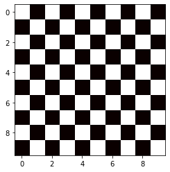
This is because $p=0$ forces the spins to always be inverted compared to the neighbour.

Let's look at what happens as we vary $p$ from 0.1 to 1.0:

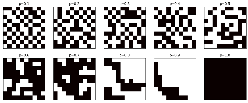
The same, on $100 \times 100$ spin glass systems:

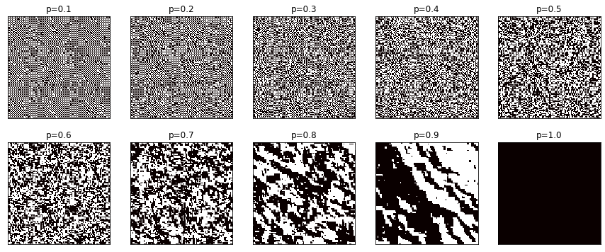
As $p$ increases, disorder increases. Note that at $p=0.5$ the neighboring spins are independent. At $p > 0.5$ domains form, because spins prefer to align with each other, but sometimes randomly an inversion occurs, and a patch is formed.

Let's check how the fraction $f$ of aligned spins varies with $p$:

rows, cols, p0 = 100, 100, 0.5
num_samples = 100
pairs = []
for p in [0.001, 0.1, 0.2, 0.3, 0.4, 0.5, 0.6, 0.7, 0.8, 0.9, 0.95, 0.975, 0.999]:
    rs = []
    for _ in range(num_samples):
        grid = create_grid(rows, cols, p0, p)
        r = np.sum(grid)/(rows*cols)
        r = max(r, 1-r)
        rs.append(r)
    pairs.append((p, np.mean(rs)))
plt.plot([x[0] for x in pairs], [x[1] for x in pairs], marker='o')
plt.xlabel('p')
plt.ylabel('f')
plt.ylim((0.48, 1.0))

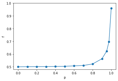
Perhaps unintuitively, the dependence is not linear. The plot has two parts:

• for $0 \leq p \leq \frac{1}{2}, f=\frac{1}{2}$. In this region, on average always half of the spins is ↑, half is ↓
  • at $p=0$, the spins are completely ordered like a chess board
  • at $p=\frac{1}{2}$, the spins are completely independent
• at $p > \frac{1}{2}$, one of the spin directions starts to dominate as $f$ breaks away from $\frac{1}{2}$, but it's very slow
  • $p$ has to get very close to 1 for $f$ to approach 1

Disorder and entropy

$f$ is constant between $0 \leq p \leq \frac{1}{2}$, but visually we can see that the system goes from order (chessboard) to complete disorder (independent spins). We can use entropy to characterize the order-disorder property of the model. Let's do brute-force Monte Carlo simulations to compute the entropy of a small $4 \times 4$ spin glass:

def entropy(frequencies, base=2):
    return -1 * sum([f/sum(frequencies) * log(f/sum(frequencies), base) for f in frequencies])

def spin_glass_entropy(rows, cols, p0, p, num_samples):
    frequencies = Counter()
    for _ in range(num_samples):
        grid = create_grid(rows, cols, p0, p)    
        frequencies[str(np.packbits(grid))] += 1
    return entropy(frequencies.values())

pairs = []
for p in [0.001, 0.1, 0.2, 0.3, 0.4, 0.5, 0.6, 0.7, 0.8, 0.9, 0.999]:
    h = spin_glass_entropy(rows=4, cols=4, p0=0.5, p=p, num_samples=100*1000)
    pairs.append((p, h))
plt.plot([x[0] for x in pairs], [x[1] for x in pairs], marker='o')
plt.xlabel('p')
plt.ylabel('entropy (bits)')
plt.ylim((0, 18))

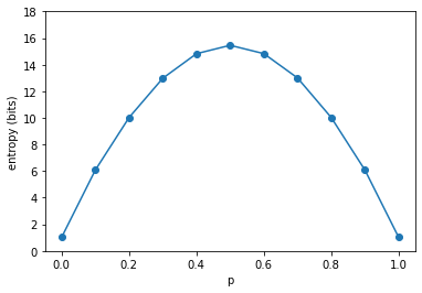
Note: the entropy shown on the y-axis is specific to this $4 \times 4$ spin glass, it would be higher for a larger system.

The entropy plot above proves our intuition: at $p=0$, the entropy is just 1 bit, which is coming from $p_0=\frac{1}{2}$, which gives two (inverted) ways to get a chess board. It's also 1 at $p=1$, where the entire spin glass is either all ↑ or all ↓. In the middle, at $p=\frac{1}{2}$, the entropy is 16 bits, since $4 \times 4 = 16$, and all the spins are independent.

The concave shape of the entropy plot is the same as that of a $p$-biased coin with entropy function $H(p)=-(p) log[p] - (1-p)log[1-p]$, so with respect to entropy the spin glass behaves like a biased coin, where the biasing factor $p$ is the correlation strength between neighboring spins.

Conclusion

Spin glasses are a widely studied models of magnetism in Physics. Here I used the toy probabilistic spin glass model to avoid having to introduce too much physical formalism (eg. Hamiltonian). We saw how the behaviour of the spin glass strongly depends on $p$, the correlation probability, and that entropy describes the order-disorder aspect of the system that we observe visually.