Random digits and Benford's law

Introduction

This is a post exploring the distribution of digits of random and non-random numbers:

1. Given a set of uniform random numbers, what is the distribution of digits?
2. How about non-random numbers, amounts like $4.95 from receipts? How close are they to random?
3. Can we reproduce Benford's law with receipt digits?

Random numbers

Let's start with random numbers. First, let's generate uniform random numbers between 0 and 1000, and look at the density plot of the numbers themselves. Left side is the histogram, right side is the cumulative histogram:

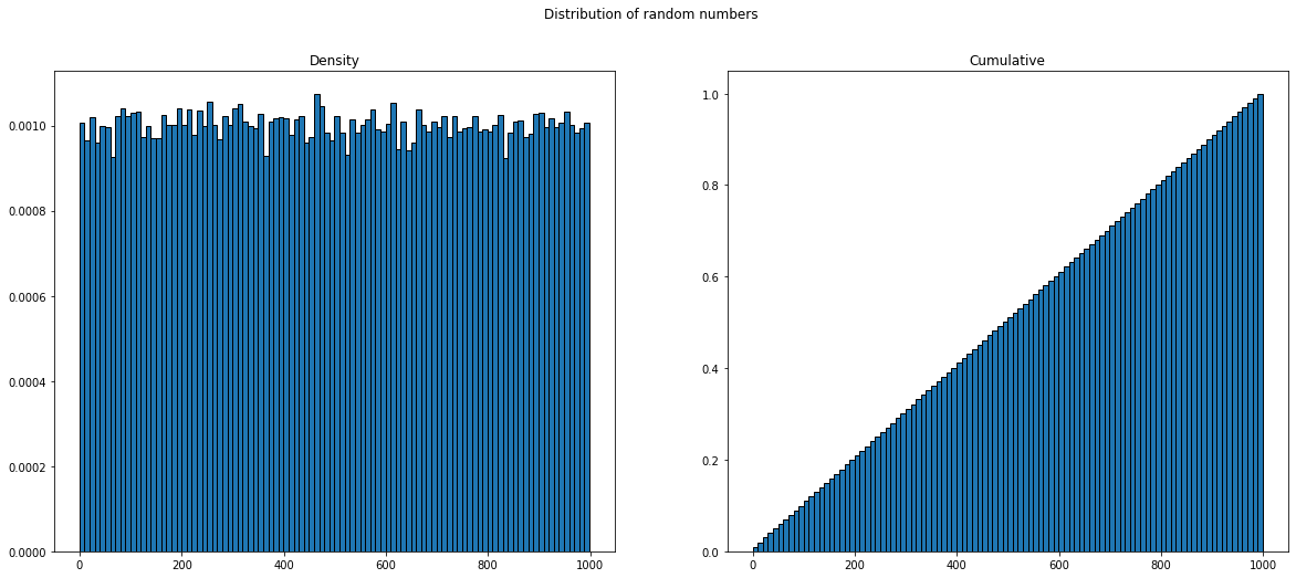
This just confirms that the code used to generate random numbers is bug-free:

num_numbers = 100*1000
upper_limit = 1000
numbers = [randint(0, upper_limit - 1) for _ in range(num_numbers)]

Now, the digits of these numbers. To get the digits, I will just use str(i), like:

plt.hist(list(map(int, list(''.join(str(i) for i in numbers)))),
         density=True, edgecolor='black', bins=list(range(0, 11)))
plt.title('Density of digits of random numbers')
plt.show()

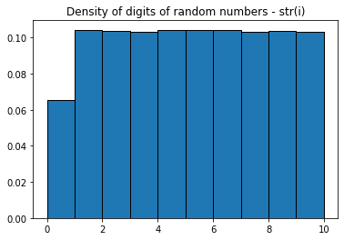
There is a deficit of 0s. This makes sense, since leading 0s are not printed with str(i), so 56 is 56 and not 056. We can "fix" this, by using '{:03d}'.format(r):

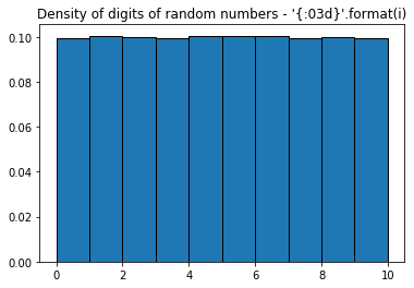
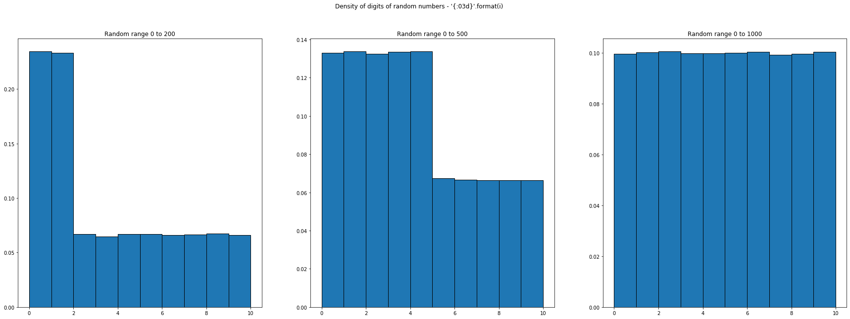
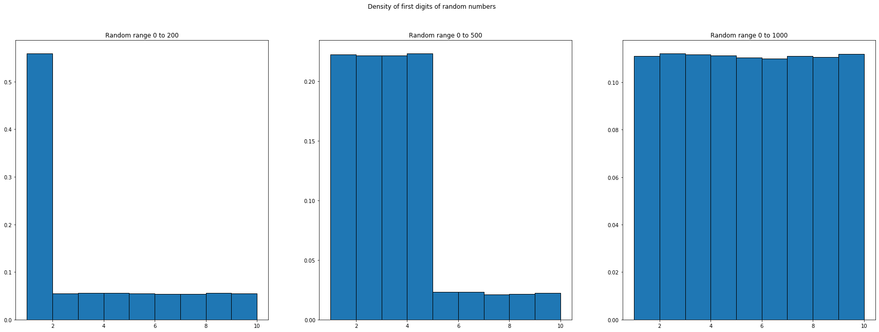
This looks right. But formatting with leading 0s doesn't neccesarily mean that the digit distribution is uniform, just because the distribution of the number is uniform — it depends on the range of the numbers. Below is the distribution of digits for even numbers drawn from different ranges 200, 500, 1000:

Finally, let's see the distribution of first digits (without leading 0s):

Amounts from receipts

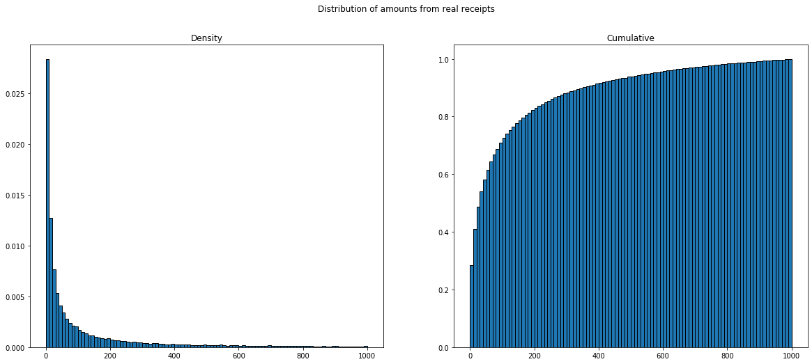
Let's leave random numbers behind, and look at amounts from real-world receipts from Dubai. Similarly as above, I cut off numbers at 1000. First, let's look at the distribution:

Next, let's look at the distribution of digits, with amounts formatted like 4.90, with 2 decimals, without leading 0s:

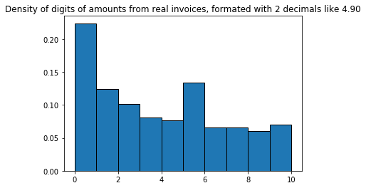
Unsurprisingly, 0 is the most frequent digit, because the decimals are often 00 or x0. What if we cut off the trailing 0s, so 4.90 becomes 4.9:

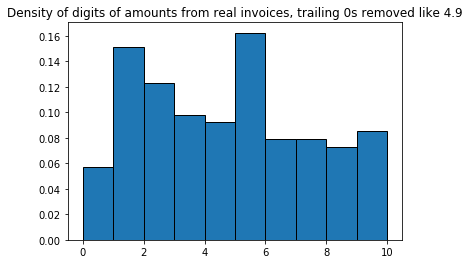
If we look at it like this, 0 is the least frequent digit, and 5 is the most frequent digit. To get a better feeling for the decimal part, we can plot the density of just the decimal numbers, so 90 from 4.90.

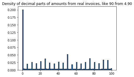
This shows that prices are likely to be multiples of 5s (like 4.00, 4.05, 4.10 ... 4.95), 00 and 50 being the most likely. Interestingly, prices are not likely to end in 9 or 99 for this dataset.

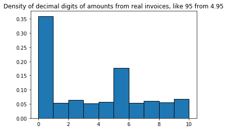
Finally, the density of digits of the decimal parts, confirming that 5 is the most likely non-zero digit:

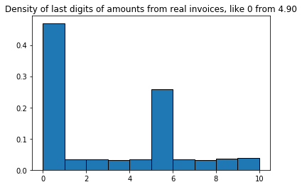
Plotting just the last digit:

Benford's law

Next, let's check Benford's law:

Benford's law, also called the Newcomb–Benford law, the law of anomalous numbers, or the first-digit law, is an observation about the frequency distribution of leading digits in many real-life sets of numerical data... It has been shown that this result applies to a wide variety of data sets, including electricity bills, street addresses, stock prices, house prices, population numbers, death rates, lengths of rivers, and physical and mathematical constants. A set of numbers is said to satisfy Benford's law if the leading digit d occurs with probability:

Plotting the distribution of first digits of our amounts, with Benford's law:

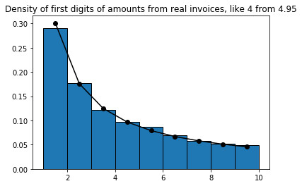
Note that first digits from uniform random numbers did not follow Benford's law, but our "real" numbers do. Interestingly, the same distributions also hold for the total amounts from receipts.

Conclusion

Digits from uniform random numbers follow a truncated-uniform distribution, depending on the formatting and upper bound. Digits from real sources like receipts and zip codes follow some artificial pattern that depends on the source, for example here the amounts tend to be multiples of 5s. Benford's law hold holds for 1st digits of "real" numbers.