Random Walks and the Dickey-Fuller Test - Part I
Marton Trencseni - Sun 20 April 2025 - Finance
Introduction
The Efficient Market Hypothesis (EMH), first articulated by Eugene Fama, asserts that asset prices fully incorporate all available information. Under the weak-form EMH, historical price and volume data cannot reliably predict future returns — implying that stock prices follow a random walk.
A symmetric random walk is recurrent: assuming the company never goes bankrupt, with probability 1 it will eventually hit any target level. In other words, in the absence of bankruptcy, a truly random walk stock price will eventually rise to any target level with probability one. That is quite interesting for an investor!
In this post, I’ll demonstrate how to apply the Dickey-Fuller test (DF) to daily price series, implement the test from scratch in NumPy, and build finite‑sample critical‑value tables via Monte Carlo simulation. The flow of the article is:
- What is the Dickey-Fuller test: intuition and hypotheses for the simplest case.
- Implementation in NumPy: coding the DF test from first principles.
- Monte Carlo simulation: building finite‑sample critical‑value tables for various series lengths.
- Visualizing the distribution: plotting the empirical PDF and CDF of the DF statistic.
- Practical examples: testing five illustrative time series to see the DF test in action.
The code is up on Github.
Dickey-Fuller test
The Dickey-Fuller test determines whether a time series $y_t$ behaves like a random walk (non-stationary) or instead is stationary (mean-reverting). The key concept is the unit root: a stochastic process has a unit root if the coefficient $\rho$ in the autoregressive model:
$y_t = \rho \cdot y_{t-1} + \epsilon_t$
satisfies $|\rho| = 1$. When $\rho = 1$, shocks $\epsilon_t$ accumulate indefinitely and the series never reverts to a fixed mean.
We define the change in the series as $\Delta y_t = y_t - y_{t-1}$. Substituting the AR(1) model yields:
$\Delta y_t = (\rho - 1) \cdot y_{t-1} + \epsilon_t = \gamma \cdot y_{t-1} + \epsilon_t$, where we defined $\gamma = \rho - 1$.
Our hypotheses are:
- The Null hypothesis H0 is: $\gamma = 0$, the series has a unit root, it is a random walk.
- Alternative hypothesis H1 is: $\gamma < 0$, the series is stationary, mean-reverting.
To test our hypotheses, we compute the t-statistic for the estimated coefficient $\hat{\gamma}$ as:
$t_{DF} = \hat{\gamma} / \sigma_{\hat{\gamma}}$
Because $y_{t-1}$ is non-stationary under H0, the resulting t-statistic follows a non-standard distribution. We therefore use Dickey-Fuller critical values (or Monte Carlo simulation) instead of standard t-tables.
In practice, this means that we run simple linear regression on the data points $\Delta y_t$ and $y_{t-1}$ per the equation $\Delta y_t = \gamma \cdot y_{t-1} + \epsilon_t$ to get the slope $\hat{\gamma}$ and the standard error of the slope estimate $\sigma_{\hat{\gamma}}$.
Code
Below is a function that computes the DF t‑statistic for a simple time series per the above:
def df_t_stat(series):
    y  = np.asarray(series, float)
    dy = np.diff(y) # Δy_t
    y1 = y[:-1]     # y_{t−1}
    # OLS slope: γ̂ = Σ y1·dy / Σ y1²
    gamma_hat = np.dot(y1, dy) / np.dot(y1, y1)
    # residuals and variance
    resid = dy - gamma_hat * y1
    T = len(y1)
    s2 = np.dot(resid, resid) / (T - 1)
    # standard error of γ̂ and DF t‑stat
    se = np.sqrt(s2 / np.dot(y1, y1))
    return gamma_hat / se
Monte Carlo simulation for critical‐value tables
To see how the DF t-statistic behaves in finite samples, we simulate many random walks of length T, compute their DF statistics, and tabulate quantiles:
def simulate_df_table(T, N=1_000_000, seed=654321):
    np.random.seed(seed)
    t_stats = np.empty(N)
    for i in range(len(t_stats)):
        rw = np.cumsum(np.random.standard_normal(T))
        t_stats[i] = df_t_stat(rw)
    # return common quantiles
    return np.percentile(t_stats, [1, 5, 10, 50, 90, 95, 99])
Then, to get a table of critical values:
quantiles = [1, 5, 10, 50, 90, 95, 99]
Ts = [50, 100, 250, 500, 1000]
table = {T: simulate_df_table(T) for T in Ts}
# header row
header = ['T'] + [f'{q}%' for q in quantiles]
row_format = '{:<5}' + ''.join('{:>10}' for _ in quantiles)
print(row_format.format(*header))
# main table
for T in Ts:
    vals = table[T]
    print(row_format.format(T, *[f'{v:.3f}' for v in vals]))
Prints something like:
T            1%        5%       10%       50%       90%       95%       99%
50       -2.619    -1.948    -1.613    -0.487     0.908     1.311     2.083
100      -2.590    -1.945    -1.615    -0.493     0.895     1.291     2.035
250      -2.570    -1.941    -1.617    -0.495     0.893     1.290     2.033
500      -2.569    -1.939    -1.617    -0.500     0.888     1.283     2.018
1000     -2.567    -1.941    -1.618    -0.500     0.888     1.281     2.017
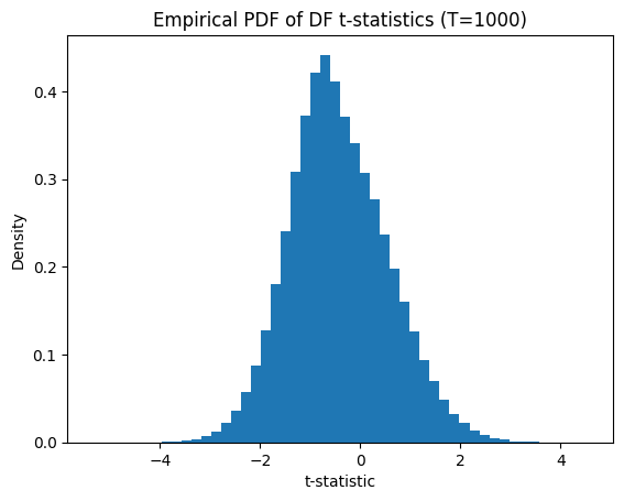
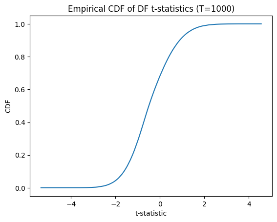
Visualizing the t-statistic distribution
Plotting the empirical distribution helps us see the non‑standard shape and heavy tails:
def simulate_t_stats(T, N=1_000_000, seed=654321):
    np.random.seed(seed)
    t_stats = np.empty(N)
    for i in range(len(t_stats)):
        rw = np.cumsum(np.random.standard_normal(T))
        t_stats[i] = df_t_stat(rw)
    return t_stats

t_stats = simulate_t_stats(T=1_000)
# empirical PDF
plt.figure()
plt.hist(t_stats, bins=50, density=True)
plt.title(f'Empirical PDF of DF t‑statistics (T={T})')
plt.xlabel('t‑statistic')
plt.ylabel('Density')
# empirical CDF
sorted_ts = np.sort(t_stats)
cdf = np.arange(1, len(sorted_ts)+1) / len(sorted_ts)
plt.figure()
plt.plot(sorted_ts, cdf)
plt.title(f'Empirical CDF of DF t‑statistics (T={T})')
plt.xlabel('t‑statistic')
plt.ylabel('CDF')
plt.show()
Examples
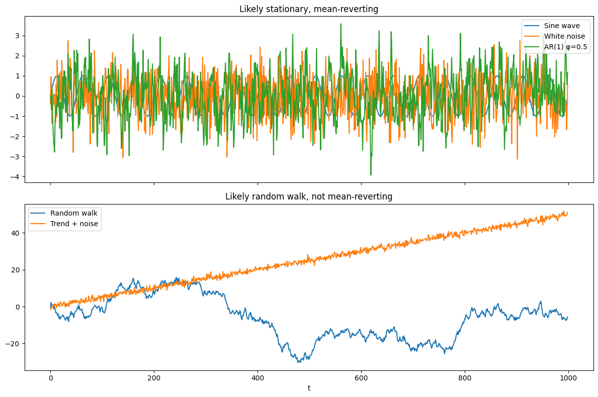
Let's look at the following time-series examples and see how our Dickey-Fuller implementation performs:
- Deterministic sine wave (periodic, non-stochastic)
- Random walk (unit root)
- White noise (i.i.d. stationary)
- Linear trend + noise (deterministic trend)
- AR(1) with φ = 0.5 (mean-reverting)
First, let's generate these time-series:
T = 1_000
t = np.arange(T)
series = {
    'Sine wave': np.sin(2 * np.pi * t / 50),                 # Deterministic sine wave (periodic, non-stochastic)
    'Random walk': np.cumsum(np.random.standard_normal(T)),  # Random walk (unit root)
    'White noise': np.random.standard_normal(T),             # White noise (i.i.d. stationary)
    'Trend + noise': 0.05 * t + np.random.standard_normal(T) # Linear trend + noise (deterministic trend)
}
# Build last: AR(1) with φ = 0.5 (mean-reverting)
phi = 0.5
ar = np.zeros_like(t, float)
for i in range(1, len(t)):
    ar[i] = phi * ar[i - 1] + np.random.standard_normal()
series['AR(1) φ=0.5'] = ar
Now, let's test each and print the conclusions, also computing the t-statistic with the statsmodel library function adfuller() to verify our implementation:
# Compute DF t-statistics, also with the library function adfuller()
results = {name: (df_t_stat(s), adfuller(s, maxlag=0, regression='n', autolag=None)[0]) for name, s in series.items()}
critical_value = simulate_df_table(T)[1]  # 5% quantile
# Print ASCII table of results
header = f"{'Series':20s} {'Our t‑stat':>12s} {'Lib t-stat':>12s} {'Reject H0? ':>12s} {'Conclusion':<40s}"
print(header)
print('-' * len(header))
for name, stat in results.items():
    reject = 'Yes' if stat[0] < critical_value else 'No'
    conclusion = 'Likely stationary, mean-reverting' if reject == 'Yes' else 'Likely random walk, not mean-reverting'
    print(f"{name:20s} {stat[0]:12.3f} {stat[1]:12.3f} {reject + ' ':>12s} {conclusion:<40s}")
Prints:
Series                 Our t‑stat   Lib t-stat  Reject H0?  Conclusion
----------------------------------------------------------------------------------------------------
Sine wave                  -1.982       -1.982         Yes  Likely stationary, mean-reverting
Random walk                -1.170       -1.170          No  Likely random walk, not mean-reverting
White noise               -30.665      -30.665         Yes  Likely stationary, mean-reverting
Trend + noise               0.289        0.289          No  Likely random walk, not mean-reverting
AR(1) φ=0.5               -17.411      -17.411         Yes  Likely stationary, mean-reverting
Our results match the library function, and all time-series were correctly classified. We can verify the latter visually:
# Group names for plotting
group1 = ['Sine wave', 'White noise', 'AR(1) φ=0.5']
group2 = ['Random walk', 'Trend + noise']
fig, (ax1, ax2) = plt.subplots(2, 1, figsize=(12, 8), sharex=True)
# Plot group 1
for name in group1:
    ax1.plot(t, series[name], label=name)
ax1.set_title('Likely stationary, mean-reverting')
ax1.legend(loc='upper right')
# Plot group 2
for name in group2:
    ax2.plot(t, series[name], label=name)
ax2.set_title('Likely random walk, not mean-reverting')
ax2.legend(loc='upper left')
ax2.set_xlabel('t')
plt.tight_layout()
plt.show()
The caveat is that the Trend + noise time-series is not an actual random walk, but it is non-stationary, not mean-reverting, which is what the Dickey-Fuller test is looking for. So if we use the DF-test as the test, we would classify it as a random walk.
Conclusion
In the next article, I will look at more sophisticated versions of the Dickey-Fuller test.