Reducing variance in A/B testing with CUPED
Marton Trencseni - Sat 31 July 2021 - ab-testing
Introduction
CUPED is a variance reduction technique introduced by Deng, Xu, Kohavi and Walker. Using CUPED we can achieve lower variance in A/B testing by computing an adjusted evaluation metric using historic "before" data. Based on blog posts, it seems that many big Internet companies are using CUPED, such as Bing, Facebook, Netflix, Booking, Etsy.
In this post I will use Monte Carlo simulations of A/B tests to demonstrate (to myself and readers) how CUPED works. The Jupyter notebook is up on Github.
Experiment setup
Assume an A/B testing setup where we're measuring a metric M, eg. $ spend per user. We have N users, randomly split into A and B. A is control, B is treatment. We have metric M for each user for the "before" time period, when treatment and control was the same, and the "after" period, when treatment had some treatment applied, which we hope increased their spend.
Let $Y_i$ be the ith user's spend in the "after" period, and $X_i$ be their spend in the "before" period, both for A and B combined. We compute an adjusted "after" spend $Y'_i$.
The CUPED recipe:
- Compute the covariance $cov(X, Y)$ of X and Y.
- Compute the variance $var(X)$ of X.
- Compute the mean $\mu_X$ of X.
- Compute the adjusted $ Y'_i = Y_i - (X_i - \mu_X) \frac{cov(X, Y)}{var(X)} $ for each user.
- Evaluate the A/B test using $Y'$ instead of $Y$.
The point of CUPED is, when using $Y'$ instead of $Y$, the estimate of the treatment lift will have lower variance, ie. on average we will be better at estimating the lift.
Mathematically, the decrease in variance will be $ \frac{var(Y')}{var(Y)} = 1 - corr(X, Y)^2 $ where $ corr(X, Y) = \frac{cov(X, Y)}{\sqrt{var(X)var(Y)}} $ is the correlation between X and Y.
Note: in some of the blog posts about CUPED, there seems to be a typo and the squared is missing from the $corr(X, Y)^2$. It's there in the original paper.
CUPED implementation
Implementing CUPED is straightforward. Assuming A_before and B_before contain the $X_i$ values for each customer in groups A and B, and A_after and B_after contain the $Y_i$ values, A_before[i] is the ith customer spend in the "before" period, A_after[i] is the same customer's "after" spend, same for the Bs. So we're indexing the users in A and B separately, the ith user in the A list (who is in group A) is a different user than the ith user in the B list (who is in group B). In code:
def get_cuped_adjusted(A_before, B_before, A_after, B_after):
    cv = cov([A_after + B_after, A_before + B_before])
    theta = cv[0, 1] / cv[1, 1]
    mean_before = mean(A_before + B_before)
    A_after_adjusted = [after - (before - mean_before) * theta for after, before in zip(A_after, A_before)]
    B_after_adjusted = [after - (before - mean_before) * theta for after, before in zip(B_after, B_before)]
    return A_after_adjusted, B_after_adjusted
Simulating one experiment
We need some code to generate the A_before, B_before, A_after, B_after lists, and in a way so that "before" and "after" are correlated. For this experiment, I chose:
- $X$ follows a normal distribution like
N(before_mean, before_sigma) - The A control $Y_i$ is the the same as $X_i$ plus a normal random variable like
N(0, eps_sigma) - The B treatment $Y_i$ is the the same as $X_i$ plus a normal random variable like
N(0, eps_sigma)plus a fixedtreatment_lift
In code:
def get_AB_samples(before_mean, before_sigma, eps_sigma, treatment_lift, N):
    A_before = list(normal(loc=before_mean, scale=before_sigma, size=N))
    B_before = list(normal(loc=before_mean, scale=before_sigma, size=N))
    A_after  = [x + normal(loc=0, scale=eps_sigma) for x in A_before]
    B_after  = [x + normal(loc=0, scale=eps_sigma) + treatment_lift for x in B_before]
    return A_before, B_before, A_after, B_after
With this, we can now run a single experiment, to see what happens with CUPED:
N = 1000
before_mean = 100
before_sigma = 50
eps_sigma = 20
treatment_lift = 2

A_before, B_before, A_after, B_after = get_AB_samples(before_mean, before_sigma, eps_sigma, treatment_lift, N)
A_after_adjusted, B_after_adjusted = get_cuped_adjusted(A_before, B_before, A_after, B_after)

print('A mean before = %05.1f, A mean after = %05.1f' % (mean(A_before), mean(A_after)))
print('B mean before = %05.1f, B mean after = %05.1f' % (mean(B_before), mean(B_after)))
print('Traditional    A/B test evaluation, lift = %.3f, p-value = %.3f' % (lift(A_after, B_after), p_value(A_after, B_after)))
print('CUPED adjusted A/B test evaluation, lift = %.3f, p-value = %.3f' % (lift(A_after_adjusted, B_after_adjusted), p_value(A_after_adjusted, B_after_adjusted)))
Yields, for example:
A mean before = 099.4, A mean after = 099.9, A mean after adjusted = 100.6
B mean before = 100.7, B mean after = 102.9, B mean after adjusted = 102.2
Traditional    A/B test evaluation, lift = 2.941, p-value = 0.214
CUPED adjusted A/B test evaluation, lift = 1.688, p-value = 0.052
So this shows that in this particular instance, the CUPED adjusted lift computed from $Y'$ (lift = 1.688) was closer to the actual lift of 2 than the traditional lift computed from $Y$ (lift = 2.941), and the p-value was lower.
If I run it a couple of times, we can also get:
A mean before = 101.8, A mean after = 102.5, A mean after adjusted = 101.9
B mean before = 100.5, B mean after = 101.7, B mean after adjusted = 102.3
Traditional    A/B test evaluation, lift = -0.854, p-value = 0.724
CUPED adjusted A/B test evaluation, lift = 0.380, p-value = 0.670
This one is quite counter-intuitive, here CUPED flipped the lift. Without CUPED, A was better than B (lift = -0.854), but with the CUPED adjustment, B is better than A (lift = 0.380). Running it a couple more times, we can also get:
A mean before = 099.5, A mean after = 099.7, A mean after adjusted = 101.6
B mean before = 103.2, B mean after = 103.4, B mean after adjusted = 101.6
Traditional    A/B test evaluation, lift = 3.743, p-value = 0.120
CUPED adjusted A/B test evaluation, lift = 0.006, p-value = 0.995
Here, CUPED adjustment made the lift estimate worse (lift = 0.006 is farther from 2 than lift = 3.743), and had a higher p-value. This is because CUPED reduces the variance on average, but not in every particular experiment instance.
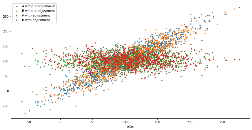
We can also visualize the original $X$ and $Y$ and adjusted $Y'$ on a scatterplot:
plt.figure(figsize=(14, 7))
plt.scatter(A_before, A_after, marker='.')
plt.scatter(B_before, B_after, marker='.')
plt.scatter(A_before, A_after_adjusted, marker='.')
plt.scatter(B_before, B_after_adjusted, marker='.')
plt.xlabel('before')
plt.xlabel('after')
plt.legend(['A without adjustment', 'B without adjustment', 'A with adjustment', 'B with adjustment'])
plt.show()
On this scatterplot, the x-axis is the "before" spend, y-axis is the "after" spend, and it's showing both $Y$ vs $X$ and $Y'$ vs $X$, for A and B, so 4 groups of points. The "linear trend" is not seasonality, it's the correlation baked in the experiment setup: somebody who spent less "before", is also likely to spend less "after", which then gets removed by CUPED:
Simulating many experiments
In order to demonstrate the variance decrease $ \frac{var(Y')}{var(Y)} = 1 - corr(X, Y)^2 $, we need to run many A/B tests, store the lifts computed using both traditional A/B testing without CUPED adjustment and with CUPED adjustment, and then compute the variances. Let's run 1,000 A/B tests and record the variances:
num_simulations = 1000
traditional_lifts, adjusted_lifts = [], []
traditional_pvalues, adjusted_pvalues = [], []
for i in range(num_simulations):
    A_before, B_before, A_after, B_after = get_AB_samples(before_mean, before_sigma, eps_sigma, treatment_lift, N)
    A_after_adjusted, B_after_adjusted = get_cuped_adjusted(A_before, B_before, A_after, B_after)
    traditional_lifts.append(lift(A_after, B_after))
    adjusted_lifts.append(lift(A_after_adjusted, B_after_adjusted))
    traditional_pvalues.append(p_value(A_after, B_after))
    adjusted_pvalues.append(p_value(A_after_adjusted, B_after_adjusted))

print('Traditional    A/B testing, mean lift = %.2f, variance of lift = %.2f' % (mean(traditional_lifts), cov(traditional_lifts)))
print('CUPED adjusted A/B testing, mean lift = %.2f, variance of lift = %.2f' % (mean(adjusted_lifts), cov(adjusted_lifts)))
print('CUPED lift variance / tradititional lift variance = %.2f' % (cov(adjusted_lifts)/cov(traditional_lifts)))
Prints:
Simulating 1000 A/B tests, true treatment lift is 2...
Traditional    A/B testing, mean lift = 2.13, variance of lift = 5.66
CUPED adjusted A/B testing, mean lift = 2.06, variance of lift = 0.80
CUPED lift variance / tradititional lift variance = 0.14
Over 1,000 A/B tests, the mean lift using traditional A/B testing (without using historic "before" data) was mean lift = 2.13 and the variance of the individual lifts about this mean was variance of lift = 5.66. The CUPED adjusted method was closer to the true mean of 2 with mean lift = 2.06 and had significantly lower variance of variance of lift = 0.80, a ratio of CUPED lift variance / tradititional lift variance = 0.14. I seperately verified that this ratio matches the theoretical exptected $ \frac{var(Y')}{var(Y)} = 1 - corr(X, Y)^2 $:
def expected_lift_ratio(A_before, B_before, A_after, B_after):
    cv = cov([A_after + B_after, A_before + B_before])
    corr = cv[0, 1] / (sqrt(cv[0, 0]) * sqrt(cv[1, 1]))
    return 1 - corr**2

large_N = 1000*1000
A_before, B_before, A_after, B_after = get_AB_samples(before_mean, before_sigma, eps_sigma, treatment_lift, large_N)
elr = expected_lift_ratio(A_before, B_before, A_after, B_after)
print('CUPED lift variance / tradititional lift variance = %.2f (expected = %.2f)' % (cov(adjusted_lifts)/cov(traditional_lifts), elr))
Prints:
CUPED lift variance / tradititional lift variance = 0.14 (expected = 0.14)
It does match, this is a good way to make sure there is no bug in the transformation code.
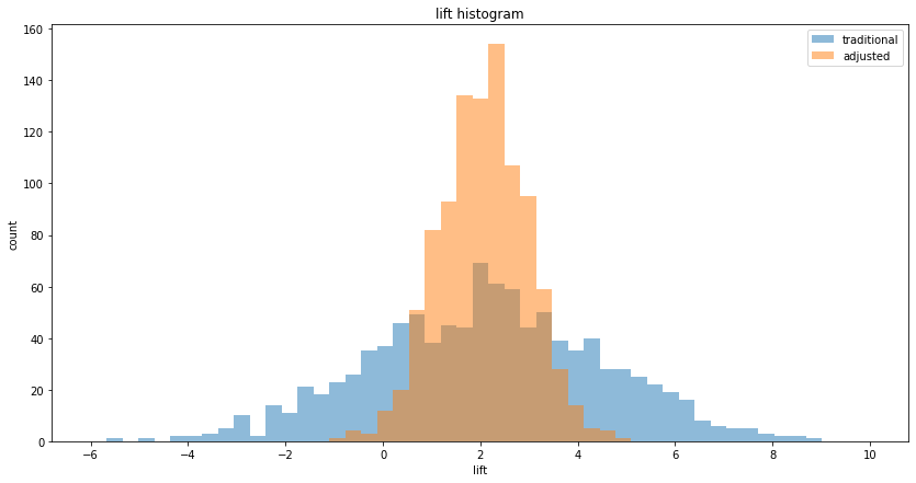
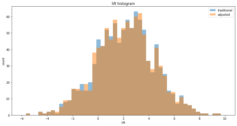
We can also plot the histogram of lifts to visualize the decrease in variance, ie. the decrease in spread:
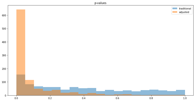
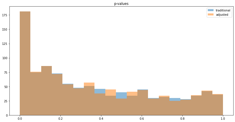
We can also visualize the histogram of p-values to see that reduced variance goes along with lower p-values:
Counter-intuitive aspects
Whether something is counter-intuitive is subjective. Below I show what I personally find counter-intuitive.
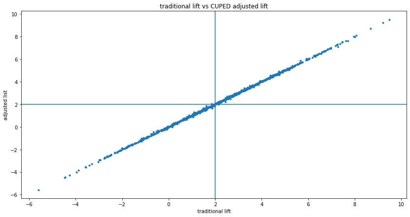
As shown in the simulation above, CUPED reduces variance on average if "before" and "after" are correlated. So in the long-run, applying CUPED is worth it. But sometimes the adjustment yields a worse measurement, which could be confusing in practice. This can be visualized by putting the traditional $Y$ and adjusted $Y'$ lift on a scatterplot, with lines showing the true lifts:
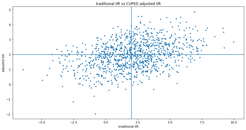
This shows that sometimes, CUPED moved the lift from better to worse, sometimes it flips it from positive to negative or negative to positive. This is not a problem, but when you get an experiment realization like this, it could be confusing.
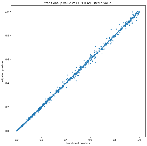
The traditional vs CUPED adjusted p-values can also be shown on a scatterplot:
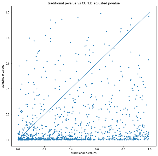
The earlier p-value histogram shows that most of the time CUPED reduces the p-value, but this shows that sometimes it increases it (experiments above the y=x line).
No correlation
Finally, let's check what happens if "before" and "after" is not correlated at all:
def get_AB_samples_nocorr(mu, sigma, treatment_lift, N):
    A_before = list(normal(loc=mu, scale=sigma, size=N))
    B_before = list(normal(loc=mu, scale=sigma, size=N))
    A_after  = list(normal(loc=mu, scale=sigma, size=N))
    B_after  = list(normal(loc=mu, scale=sigma, size=N) + treatment_lift)
    return A_before, B_before, A_after, B_after
Per the formulas, if $cov(X, Y)=0$ then CUPED does "almost nothing" in $ Y'_i = Y_i - (X_i - \mu_X) \frac{cov(X, Y)}{var(X)} $. I say "almost", because in an experiment realization the covariance will not be exactly 0, but some small number. Simulating 1,000 A/B tests confirms this:
Simulating 1000 A/B tests, true treatment lift is 2...
Traditional    A/B testing, mean lift = 2.16, variance of lift = 5.26
CUPED adjusted A/B testing, mean lift = 2.16, variance of lift = 5.25
CUPED lift variance / tradititional lift variance = 1.00
Visually:
Conclusion
CUPED is a win. It allows us to more accurately measure experimental lift if there is correlation between "before" and "after", without degrading measurements if there is not. I plan to do more posts on CUPED:
- Repeating these simulations for conversion experiments.
- Exploring how trends relate to correlation.
- Check what happens if a Data Scientist evaluates using both traditional and CUPED adjusted, and picks the more favorable outcome — I suspect this is not correct, I suspect it's "p-hacking".
Finally, some meta-commentary: in almost all the posts about A/B testing here on Bytepawn, I run Monte Carlo simulations to make sure I don't fool myself. The last post was an exception, I didn't run MC simulations, I argued "intuitively", and (mis)led myself down a rabbit hole. This is a great lesson: it's best to double-check my intuition with simulations, they are relatively quick to implement and run, worth it.