Unevenness at the edges

Introduction

Sometimes we look at the top performers in a field and see obviously uneven representations of groups (gender, ethnicity, etc). There a multitude of factors that can lead to it, such as unfair bias in access to opportunities. Here I will show one unintuitive mathematical effect that can contribute to such unevenness in the case of normal distributions.

As a toy model let's assume that there is just one metric which determines performance, such as "height" for basketball or "reaction time" for driving, and the populations are described by a normal distribution. The unintuitive effect is that even a small shift in the means of the normals (assuming equal standard deviations) can lead to a very uneven ratio at the tails.

The code is up on Github.

Normal distributions

Let's take a simple toy example, two populations A and B, both described by a normal distribution, both have standard deviations of $ \sigma = 1 $. Population A has mean $ \mu = 0 $ and B has mean $ \mu = 0.2 $, so $ A \sim \mathcal{N}(0, 1), B \sim \mathcal{N}(0.2, 1) $. This is easy to draw:

import numpy as np
import scipy.stats as stats
import matplotlib.pyplot as plt

mean_A = 0.0
mean_B = 0.2
stdev = 1
x = np.linspace(mean_A - 5, mean_A + 5, 100)
plt.plot(x, stats.norm.pdf(x, mean_A, stdev))
plt.plot(x, stats.norm.pdf(x, mean_B, stdev))
plt.show()

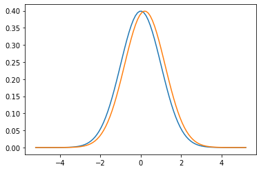
If we draw an element of A and B each at random, what's the probability that B will be "higher"?

B_taller_A = stats.norm.cdf(0, loc=mean_A-mean_B, scale=stdev)
print('%.1f' % B_taller_A)

It's 60%.

Okay, now assume that this is in fact a very large population, and we take the "top peformers". Let's take the ones above a high sigma of $ z_{cut} = 5.2 $. What will be the ratio of As to Bs at the edge of the distribution?

z_cut = 5.2
area_A = stats.norm.sf(z_cut, loc=mean_A, scale=stdev)
area_B = stats.norm.sf(z_cut, loc=mean_B, scale=stdev)
print('1 in %d' % (1/area_A))
print('1 in %d' % (1/area_B))
print('%.1f to 1' % (area_A/area_B))

This tells us that in the A population, 1 in 10,035,700 is above z_cut, in the B population it's 1 in 3,488,555, and in the end we expect the ratio of B to A to be 2.9 to 1, so roughly 3 to 1. So although Bs only have a slight edge over As in the mean, and in the overall population, at the edges we expect to see 3 times as many Bs as As! The effect becomes stronger at higher z's.

We can repeat this with real height data for males and females from Our world in data:

As an aggregate of the regions with available data – Europe, North America, Australia, and East Asia – they found the mean male height to be 178.4 centimeters (cm) in the most recent cohort (born between 1980 and 1994). The standard deviation was 7.59 cm... Women were smaller on average, with a mean height of 164.7 cm, and standard deviation of 7.07 cm.

Here we just have to do a bit more work because the standard deviations are not equal, but it's the same story. Assuming there is an equal number of males and females (a good assumption), what's the expected ratio of males to females above 185cm?

mean_A = 164.7
mean_B = 178.4
stdev_A = 7.1
stdev_B = 7.6
z_cut = 185
area_A = stats.norm.sf(z_cut, loc=mean_A, scale=stdev_A)
area_B = stats.norm.sf(z_cut, loc=mean_B, scale=stdev_B)
print('1 in %d' % (1/area_A))
print('1 in %d' % (1/area_B))
print('%.1f to 1' % (area_B/area_A))

We expect 1 in 470 females to be above 185cm, 1 in 5 males, and ratio of males to females above 185 cm is 90.7 to 1!

Exponential distributions

It's worth noting that this doesn't happen with all distributions. For example, with exponential distributions:

mean_A = 1.0
mean_B = 1.2
stdev = 0.5
z_cut = 9
area_A = stats.expon.sf(z_cut, loc=mean_A, scale=stdev)
area_B = stats.expon.sf(z_cut, loc=mean_B, scale=stdev)
print('1 in %d' % (1/area_A))
print('1 in %d' % (1/area_B))
print('%.1f to 1' % (area_B/area_A))

The unevenness at high z is only 1.5 to 1.

Causality

It's important to be careful with causality. What this shows is the mathematical fact that a shift in the mean of normal distributions leads to uneven ratios of populations at high z's. But in real life, we can't just turn it around: if we see an uneven distribution at high z's, we can't be sure if this is the reason, or some other effect. For example, currently 100% of Formula 1 drivers are male, but more than likely there are other strong determining factors, eg. parents of girls may be less likely to buy car toys, less likely to take girls gokarting at a young age, etc.