A/B testing and Multi-armed bandits
Marton Trencseni - Fri 07 August 2020 - Data
Introduction
When we perform an A/B test, we split the population in a fixed way, let's say 50-50. We then put an N number of users through the different A and B funnels: for each user, we flip a coin to decide whether they get A or B. We then measure the outcome metric for the A and B population of users, let's say conversion. We then compare the outcome metric to tell whether A or B is better. We use statistical hypothesis testing, let's say Fisher's exact test, to see whether the difference is statistically significant.
Suppose the A/B test is performed to compare different versions of signup funnels for paid licenses, so there is revenue involved. In this case, a business minded person could ask: "If B is generating more revenue than A, could we have sent less users into A and more into B, to maximize our revenue, even while the test is running?"
This is what Multi-armed bandit algorithms are for. Per Wikipedia:
In probability theory, the multi-armed bandit problem is a problem in which a fixed limited set of resources must be allocated between competing (alternative) choices in a way that maximizes their expected gain, when each choice's properties are only partially known at the time of allocation, and may become better understood as time passes or by allocating resources to the choice. This is a classic reinforcement learning problem that exemplifies the exploration–exploitation tradeoff dilemma.
In a Multi-armed bandit (MAB) approach, instead of having a fixed split of users between A and B, we make this decision based on how A and B have performed so far. MAB approaches attempt to strike a balance between exploitation (putting users into the better funnel, based on what we've seen so far) and exploration (collecting more data about funnels which have seen less users so far). In general, MAB algorithms will favor funnels which have performed better so far.
The high-level goal of MAB algorithms is to minimize regret: in this example, the additional amount of money we could have made if we put all users into the funnel that actually performs better. Here I will show three MAB algorithms: Epsilon-greedy, UCB1 and Thompson sampling.
The code shown below is up on Github.
Fixed split A/B testing
To set a baseline and write some useful code, let's start with plain-vanilla, fixed split A/B testing:
def simulate_abtest_fixed(funnels, N):
    traffic_split = [x[1] for x in funnels]
    observations = np.zeros([len(funnels), len(funnels[0][0])])
    funnels_chosen = []
    for _ in range(N):
        which_funnel = choice(traffic_split)
        funnels_chosen.append(which_funnel)
        funnel_outcome = choice(funnels[which_funnel][0])
        observations[which_funnel][funnel_outcome] += 1
    return observations, funnels_chosen
This is just regular A/B testing. It simulates N users, and each users goes into the funnels according to traffic_split:
funnels = [
    [[0.95, 0.05], 0.50], # the first vector is the actual outcomes, the second is the traffic split
    [[0.94, 0.06], 0.50],
]
N = 10*1000
num_simulations = 100
simulate_abtest_many(funnels, N, num_simulations, simulate_abtest_fixed)
We set up our experiment such that funnel A has 5% conversion, while funnel B has 6% conversion, so funnel B is better. In the context of MABs, we'd like funnel B to be chosen more often than funnel A, but we'd also like to be able to call a winner at the end decisively (with statistical significance).
The function simulate_abtest_many() is a helper function which calls the passed in experimental function (in this case, simulate_abtest_fixed()) exactly num_sumulations times, and collects statistics:
- how many times has the better funnel won
- in those cases, was the result significant
- what was the histogram of p values
- after the i-th user in the histogram, up to that point, what % of time was the user put in the better funnel B
The code for simulate_abtest_many() is:
def simulate_abtest_many(funnels, N, num_simulations, simulate_abtest_one, p_crit = 0.05):
    ps = []
    num_winning = 0
    num_significant = 0
    funnels_chosen_many = np.zeros([num_simulations, N])
    for i in range(num_simulations):
        print('Doing simulation run %d...' % i, end='\r')
        observations, funnels_chosen = simulate_abtest_one(funnels, N)
        funnels_chosen_many[i] = funnels_chosen
        if observations[1][1]/sum(observations[1]) > observations[0][1]/sum(observations[0]):
            num_winning += 1
            p = fisher_exact(observations)[1]
            if p < 0.05:
                num_significant += 1
            ps.append(p)
    print('\nDone!')
    print('Ratio better funnel won:  %.3f' % (num_winning/num_simulations))
    if num_winning > 0:
        print('Ratio of wins stat.sign.: %.3f' % (num_significant/num_winning))
        print('Histogram of p values:')
        plt.figure(figsize=(10, 5))
        ax = sns.distplot(ps, kde=False, rug=True)
        ax.set(xlabel='p value', ylabel='count')
        plt.show()
    funnels_chosen_avg = funnels_chosen_many.mean(0)
    print('Avg cumulative ratio of users in better funnel:')
    plt.figure(figsize=(10, 5))
    plt.xlabel('user sequence')
    plt.ylabel('avg cumulative ratio of users in better funnel')
    plt.plot([np.average(funnels_chosen_avg[:i]) for i in range(1, len(funnels_chosen_avg))])
Running this with a fixed split A/B test:
Ratio better funnel won:  1.000
Ratio of wins stat.sign.: 0.590
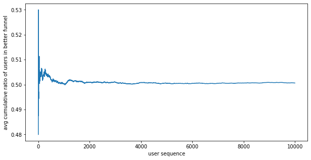
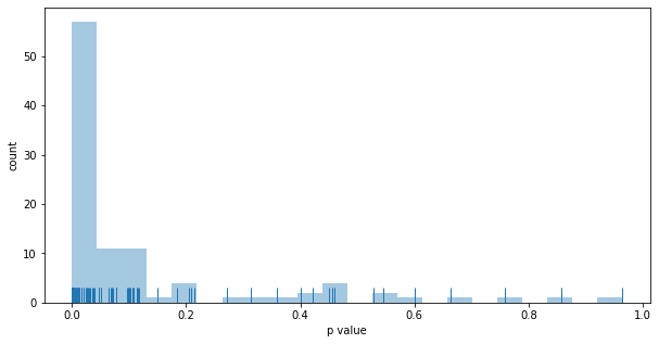
Outcomes:
- the better funnel wins 100% of the time
- the results is stat. sign. 59% of the time
- as expected, the split is 50% and doesn't change in the experiment
Epsilon-greedy
Epsilon-greedy is the simplest MAB algorithm. There is a fixed epsilon parameter, say 10%. For each incoming user, with 10% probability we randomly put the user into A or B, and with 90% probability we put them in the funnel that has performed better so far. So we explicitly control the trade-off between explore (10%) and exploit (90%). Implementation is straightforward:
def reward(observation_vector):
    if sum(observation_vector) == 0:
        return 0
    return observation_vector[1] / sum(observation_vector)

def simulate_eps_greedy(funnels, N, eps=0.1):
    explore_traffic_split = [1/(len(funnels))] * len(funnels)
    observations = np.zeros([len(funnels), len(funnels[0])])
    rewards = [0] * len(funnels)
    funnels_chosen = []
    for _ in range(N):
        if random.random() < eps:
            # explore, choose one at random
            which_funnel = choice(explore_traffic_split)
        else:
            # exploit, choose the best one so far
            which_funnel = np.argmax(rewards)
        funnels_chosen.append(which_funnel)
        funnel_outcome = choice(funnels[which_funnel])
        observations[which_funnel][funnel_outcome] += 1
        rewards[which_funnel] = reward(observations[which_funnel])
    return observations, funnels_chosen
Running the Epsilon-greedy experiment 100 times yields the following results:
Ratio better funnel won:  0.850
Ratio of wins stat.sign.: 0.376
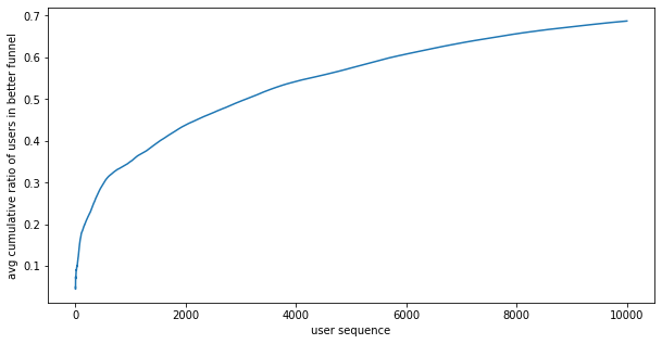
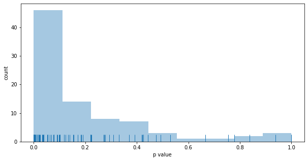
Outcomes:
- the better funnel wins 85% of the time, less than fixed A/B testing
- the results is stat. sign. 37% of the time, less than fixed A/B testing
- on average, 70% of users are put in the better funnel, better than fixed A/B testing
UCB1
UCB stands for Upper Confidence Bound. It's an algorithm that achieves regret that grows only logarithmically with the number of actions taken. For more details, see these lectures slides. The key point is that
- for each funnel $j$, maintain the conversion rate $c_j$ and number of users $n_j$
- $n$ is the total number of users so far
- choose the funnel that maximises $ c_j + \sqrt{ 2 ln(n) / n_j } $
Without going into the details, UCB1 achieves a good trade-off between exploration and exploitation. Implementation:
def ucb1_score(reward_funnel, n_funnel, n_total):
    return reward_funnel + np.sqrt(2 * np.log(n_total) / n_funnel)

def simulate_ucb1(funnels, N):
    observations = np.zeros([len(funnels), len(funnels[0])])
    # initially, set each score to a big number, so each funnel goes at least once
    ucb1_scores = [sys.maxsize] * len(funnels)
    funnels_chosen = []
    for n in range(N):
        options = [i for i, score in enumerate(ucb1_scores) if score == max(ucb1_scores)]
        which_funnel = random.choice(options)
        funnels_chosen.append(which_funnel)
        funnel_outcome = choice(funnels[which_funnel])
        observations[which_funnel][funnel_outcome] += 1
        r = reward(observations[which_funnel])
        for i in range(len(funnels)):
            if sum(observations[i]) > 0:
                r = reward(observations[i])
                ucb1_scores[i] = ucb1_score(r, sum(observations[i]), n + 1)
    return observations, funnels_chosen
Running the UCB1 experiment 100 times yields the following results:
Ratio better funnel won:  0.990
Ratio of wins stat.sign.: 0.606
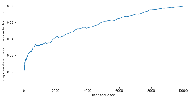
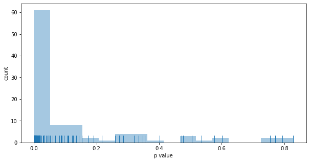
Outcomes:
- the better funnel wins 99% of the time, roughly the same as fixed A/B testing
- the results is stat. sign. 60% of the time, roughly the same as fixed A/B testing
- on average, 58% of users are put in the better funnel, somewhat better than fixed A/B testing
Thompson sampling
Thompson sampling is easy to understand if you understand how Bayesian A/B tests work and what the Beta() distribution is. The idea is simple:
- for each funnel $j$, maintain the number of converting users $C_j$ and number of users $n_j$
- for each funnel, at each incoming user, create a Beta distribution with parameters $C_j + 1$ and $n_j - C_j + 1$; the Beta distributions model the conversion % of the funnels
- draw a random number (sampled conversion) from each Beta distribution, and put the user into the funnel with the highest
The implementation is straightforward:
def beta_distributions(observations):
    return [beta(observations[i][1]+1, observations[i][0]+1) for i in range(len(observations))]

def simulate_thompson(funnels, N):
    observations = np.zeros([len(funnels), len(funnels[0])])
    funnels_chosen = []
    for n in range(N):
        betas = beta_distributions(observations)
        p_conv = [beta.rvs(1)[0] for beta in betas]
        which_funnel = np.argmax(p_conv)
        funnels_chosen.append(which_funnel)
        funnel_outcome = choice(funnels[which_funnel])
        observations[which_funnel][funnel_outcome] += 1
    return observations, funnels_chosen
Running the Thompson experiment 100 times yields the following results:
Ratio better funnel won:  0.960
Ratio of wins stat.sign.: 0.396
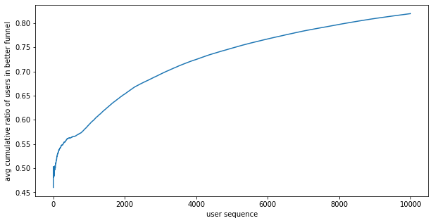
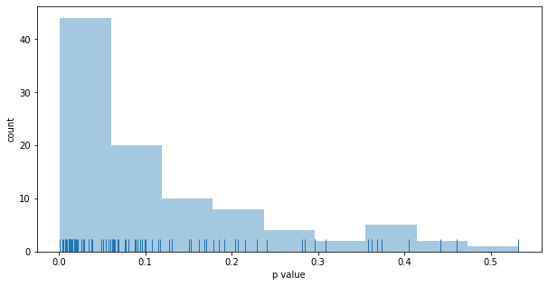
Outcomes:
- the better funnel wins 96% of the time, roughly the same as fixed A/B testing
- the results is stat. sign. 40% of the time, less than fixed A/B testing
- on average, 80% of users are put in the better funnel, better than fixed A/B testing
Conclusion
There is no free lunch. Statistical significance is a function of the funnel with the lowest number of samples, so diverting traffic from an even split yields lower significance. Different Multi-armed bandits strike a different trade-off in the space of:
- exploration (statistical significance)
- exploitation
Another aspect to consider is that Multi-armed bandits are harder to debug and understand in production. With fixed A/B testing, at any time it's possible to compare counts from exposure logs to the experiment's configuration to see if metrics are as expected. With MAB this is more involved, because we have to compare exposure log and conversion counts to the expected MAB algorithm's behaviour given the current performance. The upside is less regret (higher overall conversion).