A/B testing and the G-test
Marton Trencseni - Mon 23 March 2020 - Data
Introduction
In previous posts I discussed the $\chi^2$ test and Fisher's exact test:
Both are tests for conversion A/B testing, both can be used to test multiple funnels (A/B/C/..) with multiple outcomes (No conversion, Monthly, Annual). At low $N$, Fisher’s exact test gives accurate results, while at high $N$, the difference in $p$ values goes to zero.
The G-test is a close relative to the $\chi^2$ test, in fact the $\chi^2$ test is an approximation of the G-test. The Wikipedia page for G-test:
The commonly used $\chi^2$ tests for goodness of fit to a distribution and for independence in contingency tables are in fact approximations of the log-likelihood ratio on which the G-tests are based. The general formula for Pearson's $\chi^2$ test statistic is $ \chi^2 = \sum_i { \frac{ (O_i - E_{i} )^2 }{ E_i } } $. The approximation of G by $\chi^2$ is obtained by a second order Taylor expansion of the natural logarithm around 1. The general formula for G is $ G = 2 \sum_i { O_i \cdot \ln \frac{O_i}{E_i} } $, where $O_i$ is the observed count in a cell, $E_i$ is the expected count under the null hypothesis, $\ln$ denotes the natural logarithm, and the sum is taken over all non-empty cells.
The code for this post is on Github.
Let's reuse the contingency table example from the $\chi^2$ post:
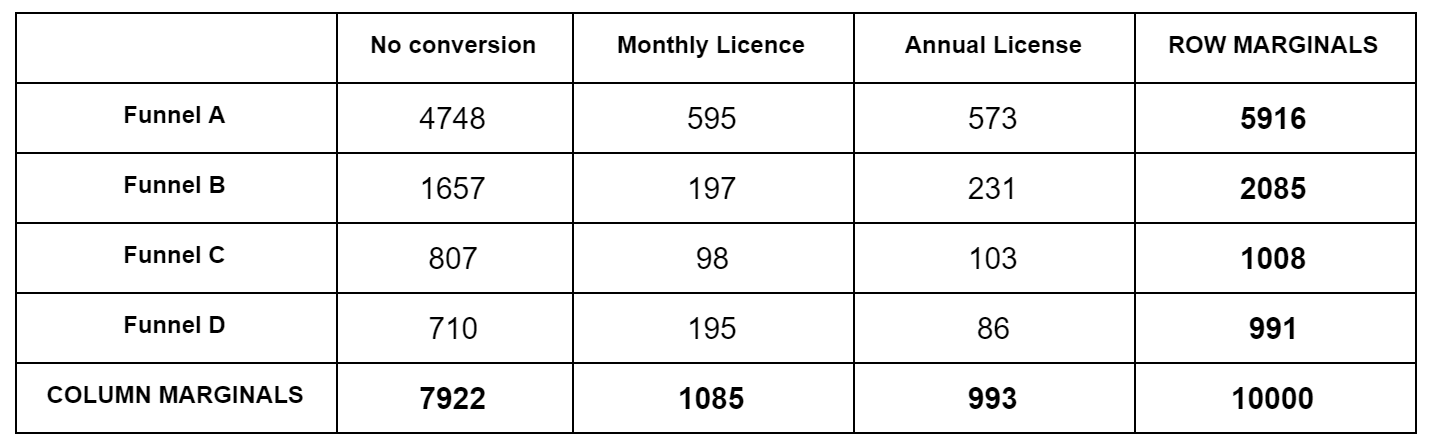
For each obsevation cell, we calculate the expected value. Expected here means according to the null hypothesis, which is that all funnels are the same. Our best guess for the null hypothesis are the blended bottom numbers: $7922/10000$ for No Conversion, $1085/10000$ for Monthly, etc. So for Funnel A, which has 5916 samples, our expected No Conversion number is $5916*7922/10000=4686.6$. We do this for each cell. Then we subtract the actual observation from the expected, square it, and divide by the expected, like $(4748-4686.6)^2/4686.6=0.8$. We do this for each cell, and sum up the numbers to we get the $\chi^2$ test statistic. We then look this up in a $\chi^2$ distribution table to get a p value. We have to use a degree of freedom of $k=(F-1)(C-1)$, where $F$ is the number of funnels, $C$ is the number of conversion events, $F=4, C=3$ above.
For the G-test, we just have to change the inner formula. Eg. for Funnel A's No Conversion case, instead of $(4748-4686.6)^2/4686.6$, we calculate $4748 \cdot \ln \frac{4748}{4686.6} $. Other than that, it's the same, add up for all cells to get the G test statistic, and look up in a $\chi^2$ distribution table to the the p value.
Because the two tests are so similar, we can write a generalized test function with a pluggable cell formula:
def generalized_contingency_independence(observations, cell_fn):
    row_marginals = np.sum(observations, axis=1)
    col_marginals = np.sum(observations, axis=0)
    N = np.sum(observations)
    chisq = 0
    for i in range(len(row_marginals)):
        for j in range(len(col_marginals)):
            expected = row_marginals[i] * col_marginals[j] / N
            chisq += cell_fn(observations[i][j], expected)
    dof = (len(row_marginals) - 1) * (len(col_marginals) - 1)
    p_value = 1.0 - chi2(dof).cdf(chisq)
    return (chisq, p_value)

def generalized_chi_squared(observations):
    return generalized_contingency_independence(observations, lambda obs, exp: (obs - exp)**2 / exp)

def generalized_G(observations):
    return generalized_contingency_independence(observations, lambda obs, exp: 2 * obs * np.log(obs / exp))
Let's simulate an A/B test where both funnels are the same (null hypothesis is true) and see the difference between the two tests:
funnels = [
    [[0.50, 0.50], 0.5], # the first vector is the actual outcomes,
    [[0.50, 0.50], 0.5], # the second is the traffic split
]
N = 1000

observations = simulate_abtest(funnels, N)
print(observations)
c_our = generalized_chi_squared(observations)
g_our = generalized_G(observations)
print('Chi-squared test statistic = %.3f' % c_our[0])
print('G test statistic = %.3f' % g_our[0])
print('Chi-squared p = %.6f' % c_our[1])
print('G p = %.6f'   % g_our[1])
Prints something like:
[[247. 278.]
 [234. 241.]]
Chi-squared test statistic = 0.490
G test statistic = 0.490
Chi-squared p = 0.483775
G p = 0.483769
We can see that the results are very close. Let's see the p value difference as a function of the sample size $N$, for different lifts for a 2x2 contingency table:
base_conversion = 0.5
traffic_split = 0.5

results = {}
for actual_lift in range(0, 10, 1):
    actual_lift /= 100.0
    results[actual_lift] = []
    for N in range(100, 10*1000, 50):
        observations = [
            [int(base_conversion * traffic_split * N), int((1-base_conversion) * traffic_split * N)],
            [int((base_conversion+actual_lift) * (1-traffic_split) * N), int((1-(base_conversion+actual_lift)) * (1-traffic_split) * N)],
        ]
        p_chi2 = generalized_chi_squared(observations)[1]
        p_g = generalized_G(observations)[1]
        p_diff = abs(p_chi2 - p_g)
        results[actual_lift].append((N, p_diff))

plt.figure(figsize=(10,5))
plt.xlabel('sample size')
plt.ylabel("""chi^2 vs G-test p difference""")
for actual_lift in results.keys():
    plt.plot([x[0] for x in results[actual_lift]], savgol_filter([x[1] for x in results[actual_lift]], 67, 3))
plt.legend(['actual_lift = %d%%' % (100*actual_lift) for actual_lift in results.keys()], loc='upper right')
plt.show()
Shows:
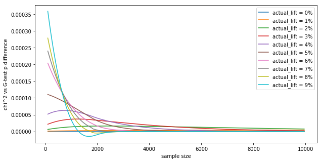
The differences in $p$ values are tiny, in the fourth decimal. In practice, this means the tests are interchangeable, as they numerically yield the same results (similar to how the t-test and z-test yield the same value numerically). This is in-line with the Wikipedia page:
For samples of a reasonable size, the G-test and the chi-squared test will lead to the same conclusions. However, the approximation to the theoretical chi-squared distribution for the G-test is better than for the Pearson's chi-squared test.
Let's see how significant the last sentence is. What this is saying is that (i) assuming the null hypothesis is true (both funnels are the same), and we (ii) perform the tests multiple times and calculate the $\chi^2$ and G test statistics, and (iii) compute the histogram of tests statistics, then (iv) the histogram of G test statistics should be a better fit to the theoretical $\chi^2$ distribution than the histogram for $\chi^2$ test statistics. This goodness of fit difference is something we can evaluate with a Monte Carlo (MC) simulation.
The simplest way computationally is to compute the 10th, 20th ... 90th percentiles of the MC test statistics, and compare that to the inverse cumulative distribution function (cdf) of the theoretical $\chi^2$ distribution taken at those percentiles. Let's run an $N=30$ A/B test 1000 times and compare the distributions:
funnels = [
    [[0.50, 0.50], 0.5], # the first vector is the actual outcomes,
    [[0.50, 0.50], 0.5], # the second is the traffic split
]
df = 1
N = 30
num_simulations = 1000

cs = []
gs = []
for _ in range(num_simulations):
    observations = simulate_abtest(funnels, N)
    cs.append(generalized_chi_squared(observations)[0])
    gs.append(generalized_G(observations)[0])

def percentiles(arr, ps):
    arr = sorted(arr)
    return [arr[int(x*len(arr))] for x in ps]

ps = [x/100.0 for x in range(1, 100, 5)]
expected_percentiles = [chi2.ppf(x, df) for x in ps]
c_percentiles = percentiles(cs, ps)
g_percentiles = percentiles(gs, ps)
plt.figure(figsize=(10,5))
plt.xlabel('percentile')
plt.xlabel('inverse cdf')
plt.plot(ps, chi2.ppf(ps, df), linestyle='--')
plt.plot(ps, c_percentiles, marker='o')
plt.plot(ps, g_percentiles, marker='x')
plt.legend(['theoretical chi^2', 'chi^2 test', 'G-test'], loc='upper left')
plt.show()
Shows:
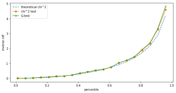
The differences are small, but we can still see them. However, such small sample sizes are unrealistic for A/B testing on the one hand, and at low sample sizes we should be using Fisher's exact test anyway. Repeating the same at $N=1,000$:
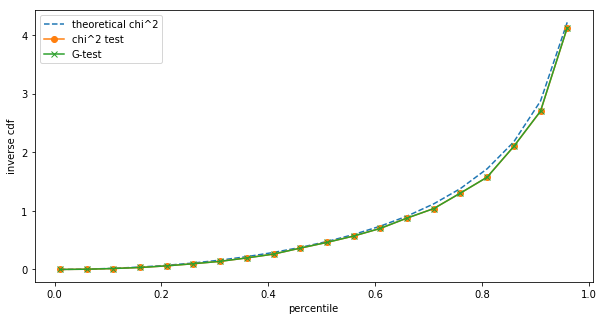
Already at $N=1,000$ we cannot see a difference between the $\chi^2$ and the G-test in terms of their test statistic distribution.
Let's do this at scale: at different $N$s, let's run num_simulations A/B tests, compute the histogram for both tests, compare to theoretical $\chi^2$ distribution, and count whether the G or the $\chi^2$ test statustic (distribution) is the better fit:
def percentile_diff(arr, percentiles, expected_percentiles):
    arr = sorted(arr)
    a_percentiles = [arr[int(x*len(arr))] for x in percentiles]
    a_diff = sum([abs(a - e) for a, e in zip(a_percentiles, expected_percentiles)])/len(expected_percentiles)
    return a_diff

def mp_fit_chi2(args):
    (num_fits, num_simulations, funnels, N, df) = args
    percentiles = [x/10.0 for x in range(1, 10, 1)]
    expected_percentiles = [chi2.ppf(x, df) for x in percentiles]
    c_diffs = []
    g_diffs = []
    for i in range(num_fits):
        cs = []
        gs = []
        for _ in range(num_simulations):
            observations = simulate_abtest(funnels, N)
            cs.append(generalized_chi_squared(observations)[0])
            gs.append(generalized_G(observations)[0])
        c_diffs.append(percentile_diff(cs, percentiles, expected_percentiles))
        g_diffs.append(percentile_diff(gs, percentiles, expected_percentiles))
    return c_diffs, g_diffs

funnels = [
    [[0.50, 0.50], 0.5], # the first vector is the actual outcomes,
    [[0.50, 0.50], 0.5], # the second is the traffic split
]
df = 1
N = 100
num_simulations = 1000
num_fits_per_thread = 500
num_threads = 24

if __name__ ==  '__main__':
    for N in [50, 100, 1000]:
        print('Running simulations for with (N, num_simulations, num_fits_per_thread) = (%s, %s, %s) on %s threads' % ((N, num_simulations, num_fits_per_thread, num_threads)))
        start_time = time.time()
        results = mp_map(
            gtest_worker.mp_fit_chi2,
            [(num_fits_per_thread, num_simulations, funnels, N, df) for _ in range(num_threads)],
            num_threads)
        elapsed_time = time.time() - start_time
        print('Done! Elapsed %s' % time.strftime("%M:%S", time.gmtime(elapsed_time)))
        c_diffs = flatten([r[0] for r in results])
        g_diffs = flatten([r[1] for r in results])
        g_better_ratio = sum([(g_diff < c_diff) for c_diff, g_diff in zip(c_diffs, g_diffs)])/len(c_diffs)
        print('The G test statistic better approximates the theoretical Chi^2 distribution %.4f fraction of times out of %s fits' % (g_better_ratio, len(c_diffs)))
        print('-')
Prints:
Running simulations for with (N, num_simulations, num_fits_per_thread) = (50, 1000, 500) on 24 threads
Done! Elapsed 29:45
The G test statistic better approximates the theoretical Chi^2 distribution 0.14 fraction of times out of 12000 fits
-
Running simulations for with (N, num_simulations, num_fits_per_thread) = (100, 1000, 500) on 24 threads
Done! Elapsed 46:45
The G test statistic better approximates the theoretical Chi^2 distribution 0.56 fraction of times out of 12000 fits
-
Running simulations for with (N, num_simulations, num_fits_per_thread) = (1000, 1000, 500) on 24 threads
Done! Elapsed 52:06
The G test statistic better approximates the theoretical Chi^2 distribution 0.48 fraction of times out of 12000 fits
The results are interesting. At $N=50$, the $\chi^2$ is actually a better fit (wins 86% of the time). At higher $N$s, it roughly the same between the two.
Conclusion
The G-test numerically yields the same results as the $\chi^2$ test, in practice it doesn't matter which one we pick for A/B tests.