Solving CIFAR-10 with Pytorch and SKL

Marton Trencseni - Tue 14 May 2019 - Machine Learning

Introduction

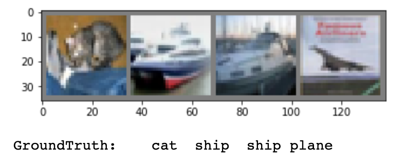
CIFAR-10 is a classic image recognition problem, consisting of 60,000 32x32 pixel RGB images (50,000 for training and 10,000 for testing) in 10 categories: plane, car, bird, cat, deer, dog, frog, horse, ship, truck. Convolutional Neural Networks (CNN) do really well on CIFAR-10, achieving 99%+ accuracy. The Pytorch distribution includes an example CNN for solving CIFAR-10, at 45% accuracy. I will use that and merge it with a Tensorflow example implementation to achieve 75%. We use torchvision to avoid downloading and data wrangling the datasets. Like in the previous MNIST post, I use SciKit-Learn to calculate goodness metrics and plots. You can run this on your laptop in a couple of hours without a GPU, the ipython notebook is up on Github.

CIFAR examples

The neural network

The CNN architecture is from this example implementation, ported to Pytorch, with log_softmax() at the final layer like in the MNIST CNN:

class CNN(nn.Module):
    def __init__(self):
        super(CNN, self).__init__()
        self.conv1 = nn.Conv2d(3,   64,  3)
        self.conv2 = nn.Conv2d(64,  128, 3)
        self.conv3 = nn.Conv2d(128, 256, 3)
        self.pool = nn.MaxPool2d(2, 2)
        self.fc1 = nn.Linear(64 * 4 * 4, 128)
        self.fc2 = nn.Linear(128, 256)
        self.fc3 = nn.Linear(256, 10)

    def forward(self, x):
        x = self.pool(F.relu(self.conv1(x)))
        x = self.pool(F.relu(self.conv2(x)))
        x = self.pool(F.relu(self.conv3(x)))
        x = x.view(-1, 64 * 4 * 4)
        x = F.relu(self.fc1(x))
        x = F.relu(self.fc2(x))
        x = self.fc3(x)
        return F.log_softmax(x, dim=1)

This time, let's automate printing out how many parameters the net has:

total = 0
print('Trainable parameters:')
for name, param in model.named_parameters():
    if param.requires_grad:
        print(name, '\t', param.numel())
        total += param.numel()
print()
print('Total', '\t', total)

Output (formatted):

Trainable parameters:

conv1.weight      1,728
conv1.bias           64
conv2.weight     73,728
conv2.bias          128
conv3.weight    294,912
conv3.bias          256
fc1.weight      131,072
fc1.bias            128
fc2.weight       32,768
fc2.bias            256
fc3.weight        2,560
fc3.bias             10
-----------------------
Total           537,610

Getting data

As mentioned, we use torchvision here:

transform = transforms.Compose([
    transforms.ToTensor(),
    transforms.Normalize((0.5, 0.5, 0.5), (0.5, 0.5, 0.5))
])

train_loader = torch.utils.data.DataLoader(
    torchvision.datasets.CIFAR10(
        root='./data',
        train=True,
        download=True,
        transform=transform),
    batch_size=4,
    shuffle=True,
    num_workers=2)

test_loader = torch.utils.data.DataLoader(
    torchvision.datasets.CIFAR10(
        root='./data',
        train=False,
        download=True,
        transform=transform),
    batch_size=4,
    shuffle=False,
    num_workers=2)

The only trick here is the normalization. The mean and standard deviation passed in is the actual value computed for the dataset, after normalization (subtract and divide) the dataset will be a standard normal N(0,1) distribution. This just helps the training.

Training the model

Training is straightforward. I've modified the code so it returns the losses, so we can plot it later:

def train(model, device, train_loader, optimizer, epoch):
    losses = []
    model.train()
    for batch_idx, (data, target) in enumerate(train_loader):
        data, target = data.to(device), target.to(device)
        optimizer.zero_grad()
        output = model(data)
        loss = F.nll_loss(output, target)
        loss.backward()
        optimizer.step()
        losses.append(loss.item())
        if batch_idx > 0 and batch_idx % 1000 == 0:
            print('Train Epoch: {} [{}/{}\t({:.0f}%)]\tLoss: {:.6f}'.format(
                epoch, batch_idx * len(data), len(train_loader.dataset),
                100. * batch_idx / len(train_loader), loss.item()))
    return losses

This is a plain vanilla training loop, with nll_loss(). This stands for negative log likelihood (NLL). NLL essentially transforms the class probability (0 to 1) to run from ∞ to 0, good for a loss function. The combination of outputing log_softmax() and minimizing nll_loss() is mathematically the same as outputing the probabilities and minimizing cross-entropy (how different are two probability distributions, in bits), but with better numerical stability.

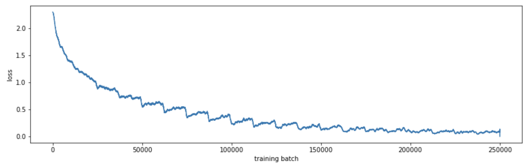
Using matplotlib we can see how the model converges:

def mean(li): return sum(li)/len(li)
plt.figure(figsize=(14, 4))
plt.xlabel('training batch')
plt.ylabel('loss')
plt.plot([mean(losses[i:i+1000]) for i in range(len(losses))])

CIFAR-10 training loss

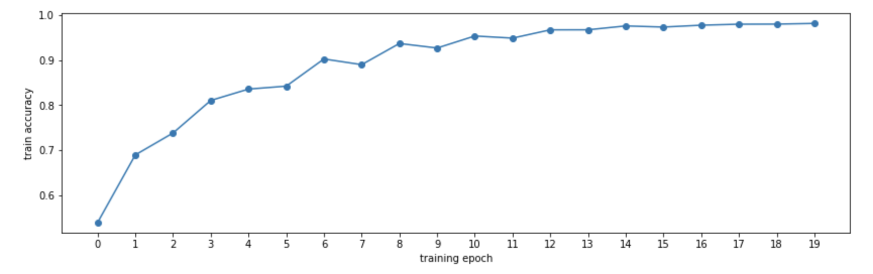
By computing the accuracy on the training set at the end of each epoch, we can see how our model improves:

CIFAR-10 training accuracy

Evaluating the model

Now we use the test data portion of CIFAR-10, and run the model on it. Most SKL metrics expect 2 of 3 inputs:

the ground truth labels
the predicted labels
the prediction probabilities (for eg. ROC curve)

Now we can use SKL to get various metrics:

def test_label_predictions(model, device, test_loader):
    model.eval()
    actuals = []
    predictions = []
    with torch.no_grad():
        for data, target in test_loader:
            data, target = data.to(device), target.to(device)
            output = model(data)
            prediction = output.argmax(dim=1, keepdim=True)
            actuals.extend(target.view_as(prediction))
            predictions.extend(prediction)
    return [i.item() for i in actuals], [i.item() for i in predictions]

actuals, predictions = test_label_predictions(model, device, test_loader)
print('Confusion matrix:')
print(confusion_matrix(actuals, predictions))
print('F1 score: %f' % f1_score(actuals, predictions, average='micro'))
print('Accuracy score: %f' % accuracy_score(actuals, predictions))

Outputs:

Confusion matrix:
[[778  20  37  12  18   6   2  25  65  37]
 [  6 854   7   5   2   4   1   1  44  76]
 [ 61   5 525  97  89  92  55  36  24  16]
 [ 20  10  32 587  65 162  45  35  19  25]
 [  9   5  34  63 715  51  41  65  13   4]
 [ 13   4  28 155  41 683  12  44   9  11]
 [  7   2  24  62  25  37 814   5  13  11]
 [ 13   3  17  38  54  61  10 785   5  14]
 [ 39   9  12  14   4   1   5   6 874  36]
 [ 23  56   6  14   4   4   5  14  35 839]]
F1 score: 0.745400
Accuracy score: 0.745400

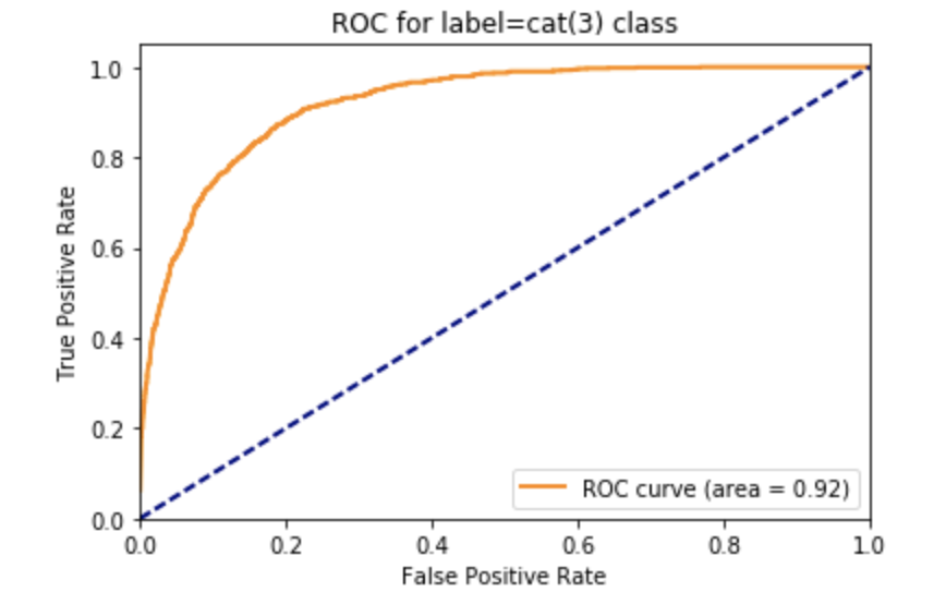
Let's see the ROC curve for the cat(3) class:

def test_class_probabilities(model, device, test_loader, which_class):
    model.eval()
    actuals = []
    probabilities = []
    with torch.no_grad():
        for data, target in test_loader:
            data, target = data.to(device), target.to(device)
            output = model(data)
            prediction = output.argmax(dim=1, keepdim=True)
            actuals.extend(target.view_as(prediction) == which_class)
            probabilities.extend(np.exp(output[:, which_class]))
    return [i.item() for i in actuals], [i.item() for i in probabilities]

which_class = 3
actuals, class_probabilities = test_class_probabilities(model, device, test_loader, which_class)

fpr, tpr, _ = roc_curve(actuals, class_probabilities)
roc_auc = auc(fpr, tpr)
plt.figure()
lw = 2
plt.plot(fpr, tpr, color='darkorange',
         lw=lw, label='ROC curve (area = %0.2f)' % roc_auc)
plt.plot([0, 1], [0, 1], color='navy', lw=lw, linestyle='--')
plt.xlim([0.0, 1.0])
plt.ylim([0.0, 1.05])
plt.xlabel('False Positive Rate')
plt.ylabel('True Positive Rate')
plt.title('ROC for label=cat(%d) class' % which_class)
plt.legend(loc="lower right")
plt.show()

CIFAR-10 ROC curve

Conclusion

While this result is not state-of-the-art, it's still much better than random, which would be 10% accuracy. I was able to run this with minimal changes from the MNIST code, since the model and the train/test framework are cleanly separated.