Warehouse locations with k-means

Introduction

Sometimes, the seven gods of data science, Pascal, Gauss, Bayes, Poisson, Markov, Shannon and Fisher, all wake up in a good mood, and things just work out. Recently we had such an occurence at Fetchr, when the Operational Excellence team posed the following question: if we could pick our KSA (=Kingdom of Saudi Arabia) warehouse locations, where would be put them? What is the ideal number of warehouses, and, what does ideal even mean? Also, what should our “delivery radius” be?

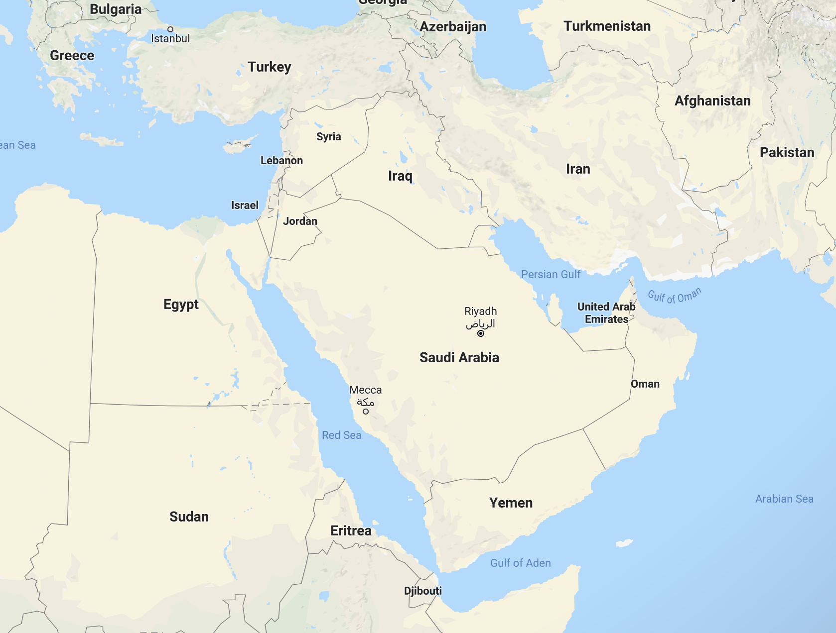
For those of us ignorant of Middle East geography, some facts about KSA:

• the biggest country in the Middle East
• mostly desert
• not very far from global conflict locations such as Iraq, Syria, Lebanon
• about 6x as big as Germany (a “big” European country), with 0.4x of the population
• about 25x as big as UAE (where Dubai, Fetchr’s HQ is)
• about 24x as big as Hungary (my home)
• responsible for 13% of the world’s oil production
• e-commerce is exploding, lots of people are ordering stuff online

Note: I will describe this fun little project as best as I can without giving away sensitive information. In some parts I will use synthetic data and in cases where the information is public/discoverable ("Fetchr has a warehouse in Riyadh"), I will just show the real thing.

Metrics and k-means

The first question is, what is “good” here? What are “good” warehouse locations? We need to find a metric to minimize/maximize. This is pretty straightforward: we need to find warehouse locations, and for each order, we assign it to the nearest warehouse (we assume it would dispatch from there), and we calculate the distance. The goal is then to find warehouse locations which minimizes the average distance across all orders.

We can write this out as a (naive) algorithm:

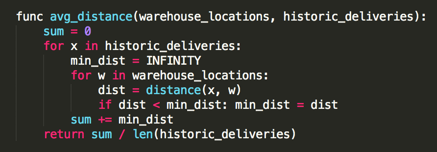
Given this choice of metric, we can evaluate a set of warehouse locations, and compare it to another.

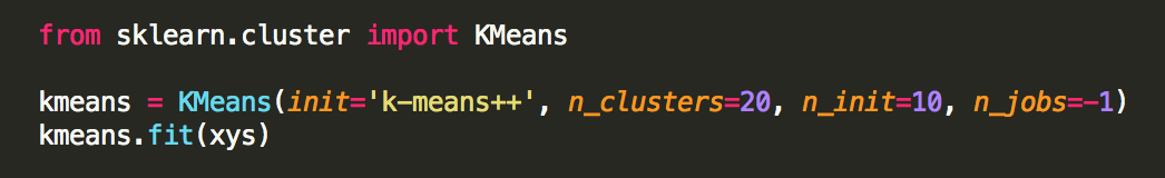
The next question is, how do we actually pick the warehouse locations? Putting aside the question of how many warehouse locations we should have, assuming we know we want N locations, there is an algorithm just for this: k-means clustering. You give k-means a set of points and a parameter N, and it returns the best N cluster centroid locations which minimizes the average distance to the nearest centroid. (This problem is actually NP-hard, so k-means returns an approximation of the solution.) At Fetchr we are standardized on Python and scikit-learn, so we used SKL’s excellent k-means implementation; it’s just 2 lines of code:

Analysis

The next question is, how do we pick N, the number of warehouses?

Note: There are other clustering algorithms such as DBSCAN that do not depend on N as an input, and tell you the best N as an output. But there is no free lunch, so even with DBSCAN you have to specifiy an epsilon parameter as an input, and it uses that epsilon to tell apart “core” and “noise” points, with clusters being dense “core” regions surrounded by sparse “noise” regions. So DBSCAN is also not parameter-free.

To keep things parameter-free and simple to interpret, we ran k-means from N = 1 .. N_max for a large N_max, and plot the average distance achieved for each N, then read off the “best value” in some sense. Later we will see that being able to vary N is actually a good thing, because we can get easy-to-interpret insights from it. So k-means it is. With this, the basic approach of our analysis is, in pseudo-code:

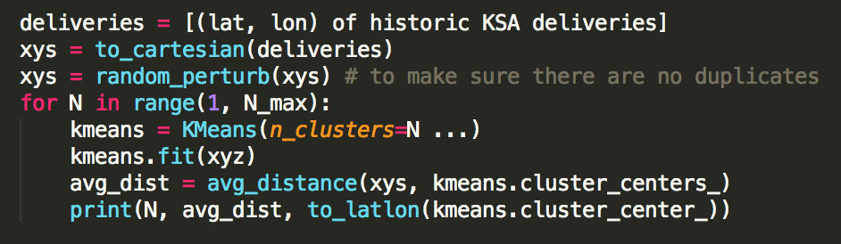
We can also compute the average distance with out actual, current KSA warehouse locations, and see how good a job the Operations team did picking them out. Running this analysis with different N, also showing actual warehouse locations, this is what the average distance curve might look like:

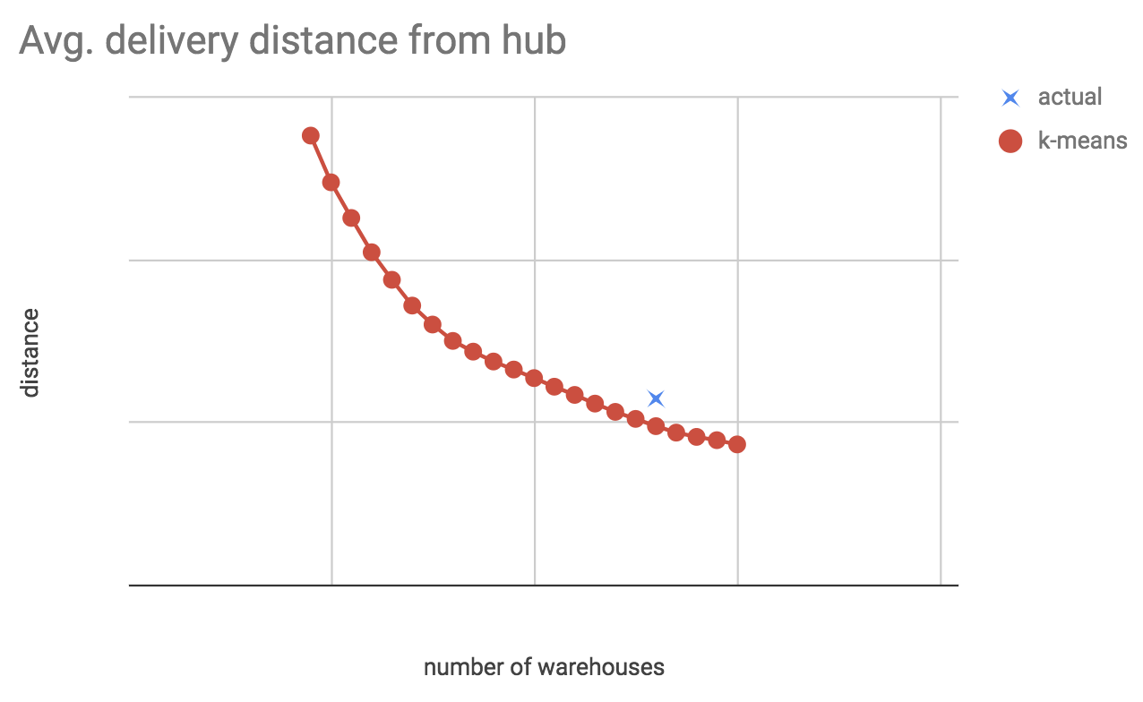
This (the real version of this) shows us:

1. How much average distance we could gain by keeping the number of hubs constant, but if we had optimal locations (move down vertically from blue cross to red line).
2. How many warehouses we could close and remain at the same average distance (move left from the blue cross to the red line).
3. Our Operations team did a good job, our current warehouse locations are pretty good.

Thinking it through, it’s obvious that the average distance will not converge to some non-zero value. It will go to zero as N (the number of warehouse locations) approaches infinity (the number of input points), since in theory we can achieve zero average distance by placing a warehouse next to each delivery location. The next best thing to check is the “derivative” of this line, ie. how much distance we “gain” (well, lose), if we add +1 warehouse. From this we will see at which N we get the biggest gains, and where the gains level off.

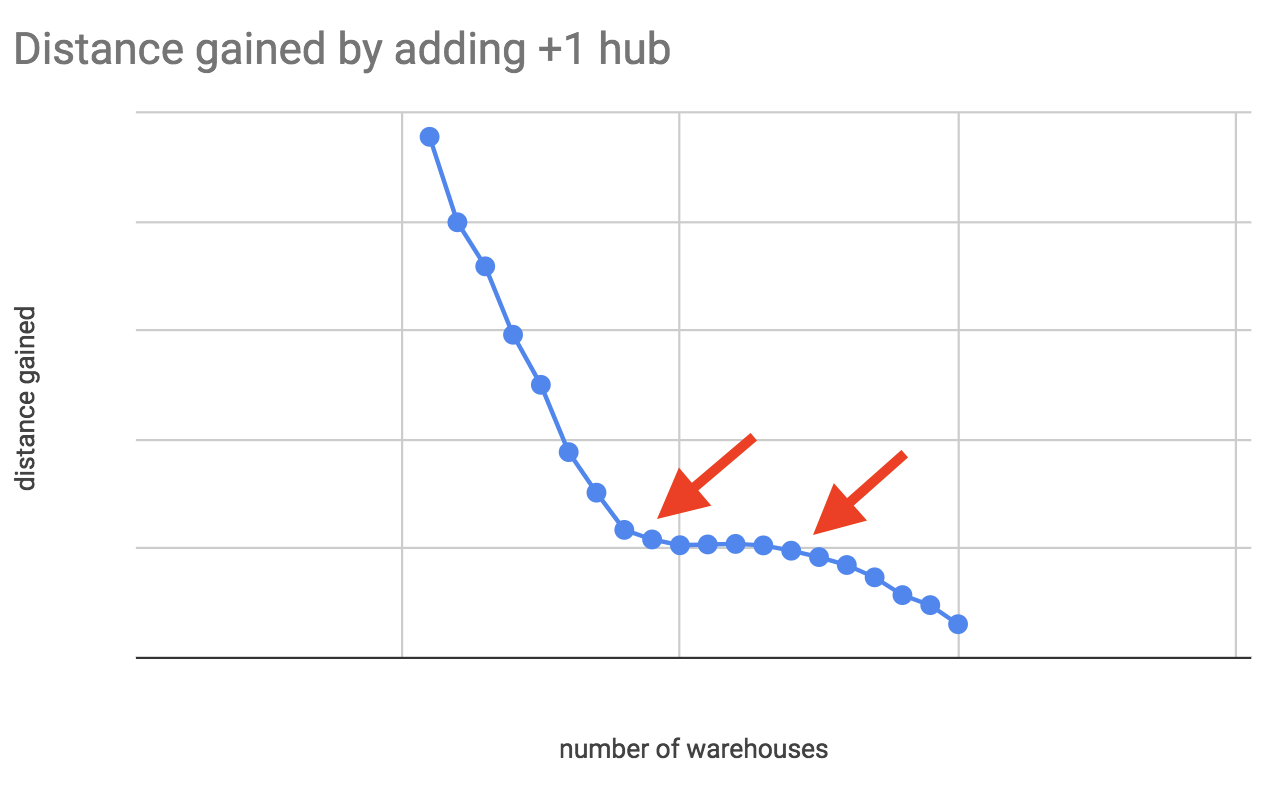
Here we can see that initially we gain a lot, then at some N our gains even out (but are non-zero). Then, a higher N the gains drop further. These are interesting points to investigate further.

With these same tools we can also investigate the question of “delivery radius”. Delivery companies often have no-service zones where they don’t accept packages, because they can’t efficiently (=profitably) service these areas. Or these areas are serviced, but only once or twice a week. To get a feel for this, we took our actual warehouse locations and put a circle of radius R kilometers around them. We investigaged as a function of the R cut-off:

1. What percentage of orders lie outside of R?
2. If we cut these outliers and re-run k-means, how much average distance do we gain?

For us, it turns out we can make a strong argument: there is a given R for which we only cut off a very low percent of orders, but we gain a lot of average distance!

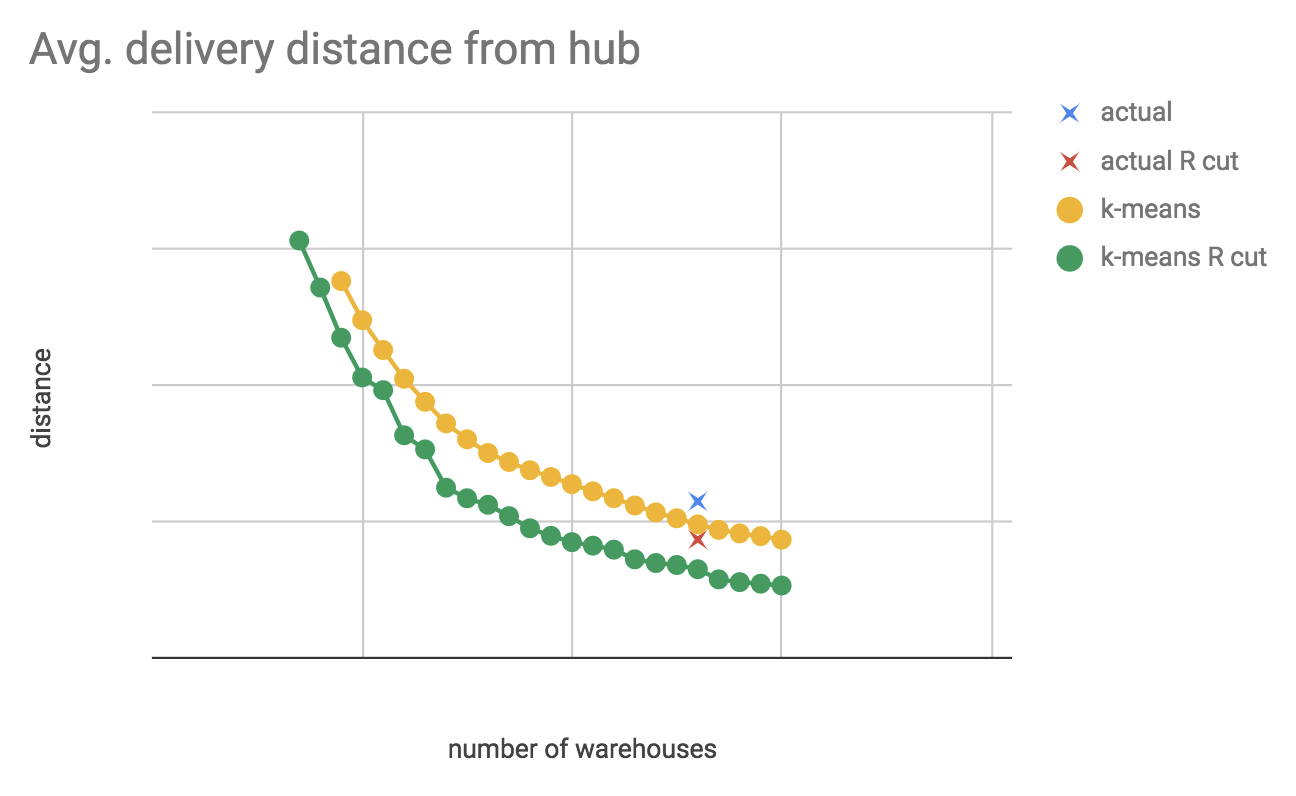
This also shows that by performing both optimizations (distance cut-off and k-means) we can actually gain a lot of efficiency; moving from the blue cross to the green line is significant. For more on outliers and outlier detection, see my previous post Beat the averages.

Locations

So far our analysis has been very quantitative in that we looked at plots and curves. We can also look at the actual recommended locations (latitude, longitude) on a map. As a starting point, we look at the k-means recommended warehouse locations when running at N = N_actual, here we expect the recommended locations to resemble our actuals; this is a sanity check on k-means. And it actually works out! For example, k-means correctly places warehouses in the center of the biggest KSA cities (eg. Riyadh, Jeddah, etc, where all medium-to-large delivery companies like Fetchr must have warehouses).

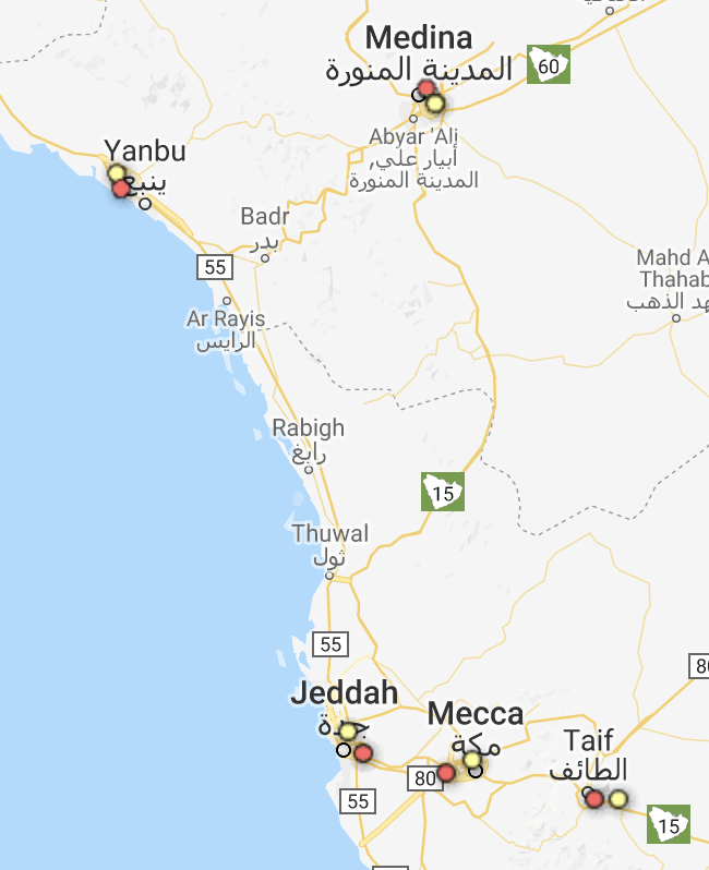
Red is actual, yellow is k-means at N = N_actual.

The interesting thing happens as we start to decrease N; essentially k-means starts finding more optimal configurations and/or recommends to merge warehouses:

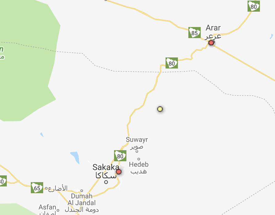
Red is actual, yellow is k-means at N < N_actual.

As we decrease N (the number of warehouses), it essentially makes recommendations, like “if you want to decrease the warehouse locations, join these two, and try to place the new one in the middle”. In real life this may or may not be feasible, because the middle may be just desert.

Conclusion and impact

This analysis was not a prescriptive (“rent N warehouses here”), it’s a discussion starter for our operations and business teams. For this reason, we can get away with using as-the-crow-flies distances instead of proper road routed distances. But still, based on this, we were able to make a good N recommendation for number of warehouses (less than actual) and locations, but we also learned that our actual warehouse locations are not too bad. We also investigated delivery radius and found that if we cut orders at a certain R distance away from a warehouse, we only cut a few % of orders, but average distance drops significantly.

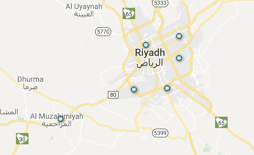
As a bonus, a few weeks later the seven gods of data science smiled on us again. It turns out there is a very similar logistics problem to picking warehouse locations: pickup locations, where customers can go and self-pickup their packages. This time, the question was: “What would the best pickup locations be in Riyadh? How many should we even have?”. We were able to re-use the same analytical framework, only this time running it on just Riyadh city data. The analysis says: "put the first 5 pickup locations into central Riyadh, and the next one into Al Muzahimiyah, the next one into... and so on."

It’s interesting that all examples on the k-means Wikipedia page are cases where the distance metric is synthetic (vector quantization, image recognition, NLP). In this beautiful logistics use-case the distance is physical Euclidian, the real thing. It’s amazing how an old-school algorithm like k-means can deliver so much impact in unexpected places!