A/B testing and the Chi-squared test
Marton Trencseni - Fri 28 February 2020 - Data
Introduction
In an ealier post, I wrote about A/B testing conversion data with the Z-test. The $\chi^2$ test is a more general test for conversion data, because it can work with multiple conversion events and multiple funnels being tested (A/B/C/D/..).
The code shown below is up on Github.
Before we go on, let’s use a $\chi^2$ test for a simple A/B conversion use-case and compare the results with the Z-test and the t-test (both two-taileds). First, a Monte Carlo algorithm to simulate A/B tests:
def choice(ps):
    return np.random.choice(len(ps), p=ps)

def simulate_abtest(funnels, N):
    traffic_split = [x[1] for x in funnels]
    observations = np.zeros([len(funnels), len(funnels[0][0])])
    for _ in range(N):
        which_funnel = choice(traffic_split)
        funnel_outcome = choice(funnels[which_funnel][0])
        observations[which_funnel][funnel_outcome] += 1
    return observations
Next, let’s pretend we’re running a conversion A/B test that’s not working (A and B conversions the same) on $N=10,000$, and use the statsmodel and scipy stats libraries to run all three tests on the results:
funnels = [
    [[0.80, 0.20], 0.6], # the first vector element is the actual outcomes,
    [[0.80, 0.20], 0.4], # the second is the traffic split
]
N = 10*1000

observations = simulate_abtest(funnels, N)
raw_data = int(observations[0][0]) * [1] + int(observations[0][1]) * [0], int(observations[1][0]) * [1] + int(observations[1][1]) * [0]
print('Observations:\n', observations)
ch = chi2_contingency(observations, correction=False)
print('Chi-sq p = %.3f' % ch[1])
zt = ztest(*raw_data)
print('Z-test p = %.3f' % zt[1])
tt = ttest_ind(*raw_data)
print('t-test p = %.3f' % zt[1])
All three yield the same p value:
Observations:
 [[4825. 1183.]
 [3211.  781.]]
Chi-sq p = 0.876
Z-test p = 0.876
t-test p = 0.876 # all three are the same
We’re not surprised that the Z-test and the t-test yield identical results. We saw in the previous post that above $N=100$ the t-distribution is a normal distribution, and the two tests yield the same p value. For this simple case (two outcomes: conversion or no conversion, and two funnels: A and B), the $\chi^2$ test is also identical to the Z-test, with the same limitation (assumes the Central Limit Theorem, so not reliable below $N=100$ ).
The $\chi^2$ test
For A/B testing, we can think of the $\chi^2$ test as a generalized Z-test. Generalized in the following sense:
- each of the funnels can have multiple outcomes, not just Conversion and No Conversion. Eg. imagine a funnel with multiple drop-off events and multiple conversions such as buying a Monthly or an Annual license (all of them mutually exclusive).
- we can test more than 2 funnel versions at once, so we can run an A/B/C/D.. test.
Let’s see this in action, eg. we have 3 outcomes and 4 funnels:
funnels = [
    [[0.80, 0.10, 0.10], 0.6], # the first vector is the actual outcomes,
    [[0.80, 0.10, 0.10], 0.2], # the second is the traffic split
    [[0.79, 0.11, 0.10], 0.1],
    [[0.70, 0.20, 0.10], 0.1],
]
N = 10*1000

observations = simulate_abtest(funnels, N)
print('Observations:\n', observations)
ch = chi2_contingency(observations, correction=False)
print('Chi-sq p = %.3f' % ch[1])
Prints something like:
Observations:
 [[4748.  595.  573.]
 [1657.  197.  231.]
 [ 807.   98.  103.]
 [ 710.  195.   86.]]
Chi-sq p = 0.000
What’s happening under the hood? Using the above 4x3 outcome table, first we construct the contingency table. We simply add the numbers row-wise and column-wise and write them at the right and bottom. These are called the marginals:
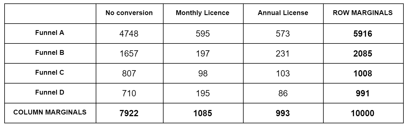
Then, for each obsevation cell, we calculate the expected value. Expected here means according to the null hypothesis, which is that all funnels are the same. Our best guess for the null hypothesis are the blended bottom numbers: $7922/10000$ for No Conversion, $1085/10000$ for Monthly, etc. So for Funnel A, which has 5916 samples, our expected No Conversion number is $5916*7922/10000=4686.6$. We do this for each cell. Then we subtract the actual observation from the expected, square it, and divide by the expected, like $(4748-4686.6)^2/4686.6=0.8$. We do this for each cell, and sum up the numbers to we get the $\chi^2$ test statistic. We then look this up in a $\chi^2$ distribution table to get a p value. We have to use a degree of freedom of $k=(F-1)(C-1)$, where $F$ is the number of funnels, $C$ is the number of conversion events, $F=4, C=3$ above.
Implementation
This is so simple, we can implement it ourselves:
def chi_squared(observations):
    row_marginals = np.sum(observations, axis=1)
    col_marginals = np.sum(observations, axis=0)
    N = np.sum(observations)
    chisq = 0
    for i in range(len(row_marginals)):
        for j in range(len(col_marginals)):
            expected = row_marginals[i] * col_marginals[j] / N
            chisq += (observations[i][j] - expected)**2 / expected
    dof = (len(row_marginals) - 1) * (len(col_marginals) - 1)
    p_value = 1.0 - chi2(dof).cdf(chisq)
    return (chisq, p_value)
We can verify we calculate the same test statistic and p value as the library function:
funnels = [
    [[0.80, 0.10, 0.10], 0.6], # the first vector is the actual outcomes,
    [[0.80, 0.10, 0.10], 0.2], # the second is the traffic split
    [[0.80, 0.10, 0.10], 0.1],
    [[0.80, 0.10, 0.10], 0.1],
]
N = 10*1000

observations = simulate_abtest(funnels, N)
print('Observations:\n', observations)
ch_scipy = chi2_contingency(observations, correction=False)
ch_our = chi_squared(observations)
print('Statsmodel chi-sq test statistic = %.3f' % ch_scipy[0])
print('Our chi-sq test statistic        = %.3f' % ch_our[0])
print('Statsmodel chi-sq p = %.3f' % ch_scipy[1])
print('Our chi-sq p        = %.3f' % ch_our[1])
Prints something like:
Observations:
 [[4846.  594.  591.]
 [1628.  188.  171.]
 [ 767.  100.   98.]
 [ 824.   84.  109.]]
Statsmodel chi-sq test statistic = 7.324
Our chi-sq test statistic        = 7.324
Statsmodel chi-sq p = 0.292
Our chi-sq p        = 0.292
Intuition
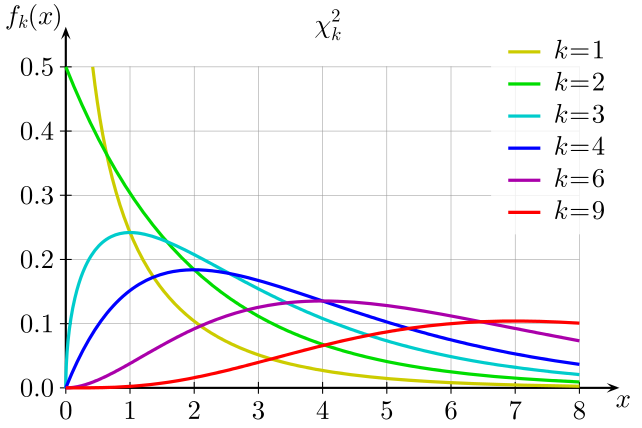
The intuition behind the $\chi^2$ is this: if the null hypothesis is true, then all rows should follow the same conversion ratios, which is also the marginal conversion ratio vector. When we subtract the expected number from the actual number (and normalize), similar to the Z-test, we get a standard normal variable. Since we have multiple cells, we need to add these variables to get an overall statistic, but we don’t want positive and negative fluctuations to cancel out. Hence we first square, and then add. So the $\chi^2$ is a sum of squares of standard normals. This is exactly what the $\chi^2$ distribution is: a $\chi^2$ distribution with degree of freedom $k$ is the result of adding up $k$ independent standard normal variables squared. In the subsequent discussion we will get more intuition why the degree of freedom is $k=(F-1)(C-1)$. Note that the standard normal goes from $-\infty$ to $\infty$, but the $\chi^2$, being its square, goes from $0$ to $\infty$. This has implications for one-tailed vs two-tailed testing.
In the 2x2 case, why is this exactly the same as the z-test? The answer is simple: in the 2x2 case, the degree of freedom is 1, the $\chi^2$ test is doing exactly the same thing as a 2-sided Z-test, and in fact the $\chi^2$ test statistic in this case is $z^2$. We can see this numerically:
funnels = [
    [[0.80, 0.20], 0.6], # the first vector is the actual outcomes,
    [[0.80, 0.20], 0.4], # the second is the traffic split
]
N = 10*1000

observations = simulate_abtest(funnels, N)
raw_data = int(observations[0][0]) * [1] + int(observations[0][1]) * [0], int(observations[1][0]) * [1] + int(observations[1][1]) * [0]
print('Observations:\n', observations)
ch = chi2_contingency(observations, correction=False)
print('Chi-sq test statistic = %.3f' % ch[0])
print('Chi-sq p = %.3f' % ch[1])
zt = ztest(*raw_data)
print('Z-test z = %.3f' % zt[0])
print('Z-test z^2 = %.3f' % zt[0]**2)
print('Z-test p = %.3f' % zt[1])
Prints something like:
Observations:
 [[4836. 1193.]
 [3147.  824.]]
Chi-sq test statistic = 1.378
Chi-sq p = 0.240
Z-test z = 1.174
Z-test z^2 = 1.378 # z^2 is the same as the Chi-sq test statistic
Z-test p = 0.240
If you compare the $\chi^2$ formulas with the Z-test formulas from the previous post, it works out that $z^2 = \chi^2$.
One-tailed vs two-tailed
In the case of the Z-test (and t-test), we have a choice between a one-tailed and a two-tailed test, depending on if we want the test to go off for deviations in just one or both directions. In the case of the $\chi^2$ test, we do not have a choice:
- the $\chi^2$ distribution is asymmetric (from $0$ to $\infty$), so technically the $\chi^2$ test is always one-tailed
- however, since it’s the square of normals, both tails of the normal are folded together, so it corresponds to a two-tailed Z-test [in the 2x2 case]
- this is not just a mathematical artefact; when dealing with multiple conversion events, there is no such thing as “positive” and “negative” directions; for example, in a 2x3 conversion example, if the baseline is $80-10-10$ for No Conversion - Monthly - Annual, and our test comes out at $79-11-10$ or $79-10-11$, which is “positive” and “negative”? (If both are “positive”, then merge the conversions, and do a 2x2 one-tailed Z-test (or t-test)).
We can check this simply:
funnels = [
    [[0.80, 0.20], 0.6], # the first vector is the actual outcomes,
    [[0.80, 0.20], 0.4], # the second is the traffic split
]
N = 10*1000

observations = simulate_abtest(funnels, N)
raw_data = int(observations[0][0]) * [1] + int(observations[0][1]) * [0], int(observations[1][0]) * [1] + int(observations[1][1]) * [0]
print('Observations:\n', observations)
ch = chi2_contingency(observations, correction=False)
print('Chi-sq p = %.3f' % ch[1])
zt = ztest(*raw_data, alternative='two-sided')
print('Z-test p (Two-tailed) = %.3f' % zt[1])
tt = ttest_ind(*raw_data, alternative='two-sided')
print('t-test p (Two-tailed) = %.3f' % zt[1])
zt = ztest(*raw_data, alternative='larger')
print('Z-test p (One-tailed) = %.3f' % zt[1])
tt = ttest_ind(*raw_data, alternative='larger')
print('t-test p (One-tailed) = %.3f' % zt[1])
Prints something like:
Observations:
 [[4780. 1181.]
 [3243.  796.]]
Chi-sq p              = 0.898 # the first three are the same
Z-test p (Two-tailed) = 0.898
t-test p (Two-tailed) = 0.898
Z-test p (One-tailed) = 0.551 # these are different
t-test p (One-tailed) = 0.551
Degrees of freedom
When we're doing hypothesis testing, we're computing a p value. The p value is the probability that we'd get the measured outcome, or more extreme outcomes, assuming the null hypothesis is true. There is one caveat here, hidden in the "or more extreme": the statistically correct way to evaluate this "more extreme" part is by keeping both row and column marginals fixed. Ie. what are all the ways (their probabilities) that we can put different numbers in the contingency table, while keeping the marginals fixed. Although the $\chi^2$ is not calculating this probability directly, thanks to the CLT, this is in fact what it's approximating in the $N \rightarrow \infty$ limit. And given a $F \times C$ table with the marginals fixed, you can only change $(F-1)(C-1)$ numbers freely ("degrees of freedom"), the rest are fixed by the constraint that the rows and columns have to add up to the marginals.
In the next post, I will talk about Fisher's exact test, which will give more intuition about this, because that test explicitly calculates this probability.
Conclusion: usage and limitations
Z-test. In the 2x2 case, the $\chi^2$ test yields exactly the same results as a two-tailed Z-test (or t-test).
Central Limit Theorem. Like the Z-test, we need enough sample size for the normal approximation to be correct. I would not be comfortable unless each cell in the contingency table is at least $X>100$. See earlier post A/B Testing and the Central Limit Theorem.
Multiple funnels, multiple outcomes. Unlike the Z-test, the $\chi^2$ test can test multiple funnels and multiple outcomes at the same time.
One-tailed distribution. Unlike the Z-test, the $\chi^2$ test is directionless (technically one-tailed, but corresponds to the two-tailed Z-test in the 2x2 case).
Degrees of freedom. For a test with $F$ funnels and $C$ outcomes you have to use the $k=(F-1)(C-1)$ degree of freedom $\chi^2$ distribution to look up the p value.