Comparing NeuralProphet and Prophet for timeseries forecasting
Marton Trencseni - Tue 20 July 2021 - modeling
Introduction
In the last past I ran forcasting experiments with Prophet. In the conclusion I mentioned NeuralProphet, a Pytorch and neural network based alternative to Prophet.
An overview of the NeuralProphet architecture from the documentation:
NeuralProphet is a decomposable time series model with the components, trend, seasonality, auto-regression, special events, future regressors and lagged regressors. Future regressors are external variables which have known future values for the forecast period whereas the lagged regressors are those external variables which only have values for the observed period. Trend can be modelled either as a linear or a piece-wise linear trend by using changepoints. Seasonality is modelled using fourier terms and thus can handle multiple seasonalities for high-frequency data. Auto-regression is handled using an implementation of AR-Net, an Auto-Regressive Feed-Forward Neural Network for time series. Lagged regressors are also modelled using separate Feed-Forward Neural Networks. Future regressors and special events are both modelled as covariates of the model with dedicated coefficients.
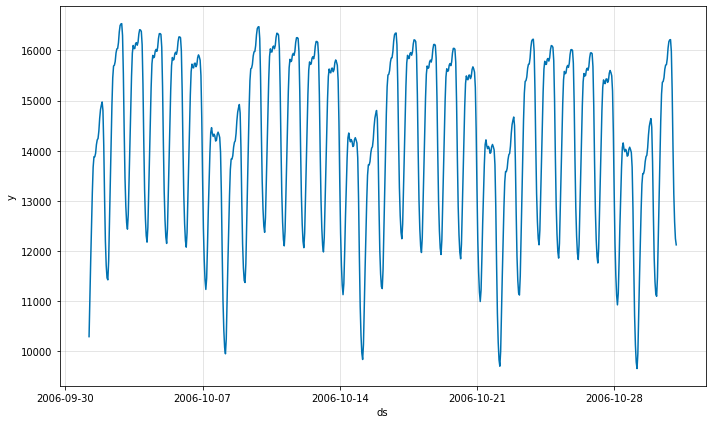
Here I will compare Prophet and NeuralProphet forecast and runtime performance. As in the previous post, let's use a sample timeseries dataset which contains hourly energy usage data for the major US energy company American Electric Power(AEP), in megawatts. We expect this timeseries to have daily and weekly seasonality, so it's an ideal candidate for forecasting.
The notebook for this post is on Github.
Getting started with NeuralProphet
Getting started with NeuralProphet is easy, the library interfaces are similar to Prophet, though, unfortunately, not identical:
# download data
df = pd.read_csv('https://github.com/khsieh18/Time-Series/raw/master/AEP_hourly.csv')
# rename columns, NeuralProphet expects ds and y
df.columns = ['ds', 'y']
df['ds'] = df['ds'].astype('datetime64[ns]')
# keep training data
training_days = 2*365
forecast_days = 30
df = df.sort_values(['ds']).head(training_days * 24)
df.index = np.arange(0, len(df))
# train model
model = NeuralProphet(yearly_seasonality=True)
model.fit(df, freq="H")
# forecast
df_predict = model.make_future_dataframe(df, periods=forecast_days * 24)
df_predict = model.predict(df_predict)
fig = model.plot(df_predict)
Yields:
NeuralProphet vs Prophet forecast performance
Let's compare NeuralProphet vs Prophet forecast performance, in terms of Mean Absolute Percentage Error (MAPE) and running time (in seconds, training and forecasting time combined, on an 8-core 64GB Intel Macbook Pro). For both MAPE and runtime, lower is better. The following helper functions have the core logic:
def compute_mape(df, df_predict, forecast_days):
    df_cross = df.tail(forecast_days*24).merge(right=df_predict, on='ds', suffixes=['', '_predict'])
    df_cross = df_cross[['ds', 'gt', 'yhat']]
    mape = mean([2 * abs((row['gt'] - row['yhat']) / (row['gt'] + row['yhat'])) for _, row in df_cross.iterrows()])
    return mape

def prepare_dfs(csv_path, training_days, forecast_days, drop_ratio=0.0):
    df = pd.read_csv(csv_path)
    # rename columns, Prophet expects ds and y
    df.columns = ['ds', 'y']
    df['ds'] = df['ds'].astype('datetime64[ns]')
    df = df.sort_values(['ds']).head((training_days + forecast_days) * 24)
    df.index = np.arange(0, len(df))
    # save ground truth
    df['gt'] = df['y']
    # wipe target variable y for to-be-forecasted section
    for i, row in df.iterrows():
        if i >= training_days * 24:
            df.at[i, 'y'] = None
    drop_inds = [i for i in range(len(df)) if random() < drop_ratio and i < len(df) - forecast_days * 24]
    df = df.drop(df.index[drop_inds])
    df_train = df.dropna()[['ds', 'y']]
    return df, df_train

def fbprophet_test(model, csv_path, training_days, forecast_days, drop_ratio=0.0):
    df, df_train = prepare_dfs(csv_path, training_days, forecast_days, drop_ratio)
    model.fit(df_train)
    df_predict = df[['ds']]
    df_predict = model.predict(df_predict)[['ds', 'yhat']]
    return compute_mape(df, df_predict, forecast_days)

def neuralprophet_test(model, csv_path, training_days, forecast_days, drop_ratio=0.0):
    df, df_train = prepare_dfs(csv_path, training_days, forecast_days, drop_ratio)
    model.fit(df_train, freq="H")
    df_predict = model.make_future_dataframe(df_train, periods=forecast_days * 24)
    df_predict = model.predict(df_predict)[['ds', 'yhat1']].rename(columns={'yhat1': 'yhat'})
    return compute_mape(df, df_predict, forecast_days)
The differences between fbprophet_test() and neuralprophet_test() show the minor differences between the two forecasting APIs.
Let's compare training on 1, 2, 3, 4, 5 years of hourly data and forecasting on 1, 3, 6, 9, 12 months of hourly data:
df = pd.read_csv('https://github.com/khsieh18/Time-Series/raw/master/AEP_hourly.csv')
training_years = [1, 2, 3, 4, 5]
forecast_months = [1, 2, 3, 6, 9, 12]
models = [
    (lambda: Prophet(yearly_seasonality=True), fbprophet_test),
    (lambda: NeuralProphet(yearly_seasonality=True), neuralprophet_test),
]
results = []
for ty in training_years:
    for fm in forecast_months:
        for funcs in models:
            training_days = int(ty * 365)
            forecast_days = int(fm * 30)
            start = time.time()
            model = funcs[0]()
            test_func = funcs[1]
            mape = test_func(model, csv_path, training_days, forecast_days)
            elapsed = time.time() - start
            print('%s, training years=%d, forecast months=%d, MAPE = %.2f, elapsed secs = %.2f' % (model.__class__.__name__, ty, fm, mape, elapsed))
            results.append((model.__class__.__name__, ty, fm, mape, elapsed))
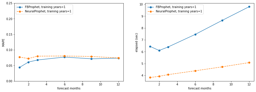
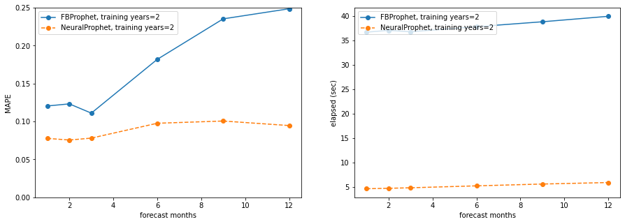
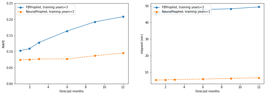
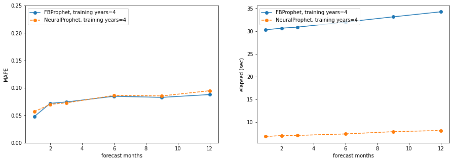
Plotting the results, both in terms of MAPE and runtime (seconds), lower is better for both. On all plots, the x-axis is forecasting months (from 1 to 12), on the left side plots the y-axis is MAPE (all axes go from 0 to 0.25), the right side plots show runtime seconds (not 0 grounded):
training_years = 1
training_years = 2
training_years = 3
training_years = 4
training_years = 5
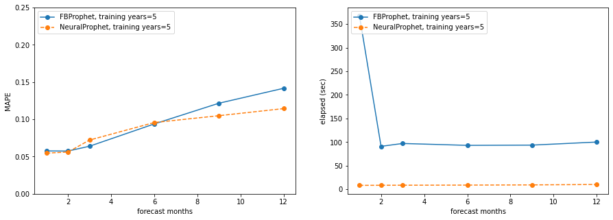
Takeaways:
- NeuralProphet is significantly faster than Prophet, even running on a Macbook Pro without GPU support for Pytorch
- NeuralProphet has lower (better) MAPE in most cases
Handling missing data
Let's fix training years at 5 and forecast months at 6, but vary the drop ratio between 0.0 and 0.5. meaning that at most 50% of all training rows are dropped, and let's see how MAPE varies:
df = pd.read_csv('https://github.com/khsieh18/Time-Series/raw/master/AEP_hourly.csv')
ty = 5
fm = 6
drop_ratios = [0.0, 0.1, 0.2, 0.3, 0.4, 0.5]
models = [
    (lambda: Prophet(yearly_seasonality=True), fbprophet_test),
    (lambda: NeuralProphet(yearly_seasonality=True), neuralprophet_test),
]
results2 = []
for drop_ratio in drop_ratios:
    for funcs in models:
        training_days = int(ty * 365)
        forecast_days = int(fm * 30)
        start = time.time()
        model = funcs[0]()
        test_func = funcs[1]
        mape = test_func(model, csv_path, training_days, forecast_days, drop_ratio)
        elapsed = time.time() - start
        print('%s, training years=%d, forecast months=%d, MAPE = %.2f, elapsed secs = %.2f, drop_ratio=%.1f'
            % (model.__class__.__name__, ty, fm, mape, elapsed, drop_ratio))
        results2.append((model.__class__.__name__, ty, fm, mape, elapsed, drop_ratio))
print('\nDone!')
Yields:
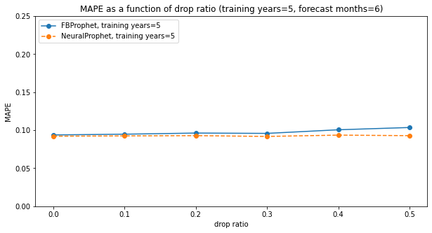
Interestingly, neither Prophet or NeuralProphet is affected by dropping up to 50% of rows. NeuralProphet does a slightly better job at higher drop_ratios.
Conclusion
This toy benchmark is not conclusive, but it indicates that NeuralProphet is competitive with Prophet on MAPE, and much faster in terms of runtime. Since NeuralProphet is quite similar to Prophet and easy to use, it's worth checking out for real life production use-cases to save time and possibly gain a few MAPE points.