Estimating mathematical constants with Monte Carlo simulations

Marton Trencseni - Sun 09 October 2022 - Monte Carlo

Introduction

Over the past years I've written many blog posts where I used Monte Carlo simulations to compute a quantity or illustrate a concept. A Monte Carlo simulation is just a simulation involving random numbers. Usually it's involved when directly computing a quantity is not feasible, but it can efficiently be estimated by some random method. Typically, estimation with Monte Carlo simulations becomes more accurate the longer we run it.

Past articles using Monte Carlo simulations:

Here I will use simple (<10 LOC) Monte Carlo simulations to estimate famous mathematical constants: $\sqrt{2}, \phi, e$ and $\pi$. The code is on Github.

Estimate $\sqrt{2}$

$\sqrt{2}$ is the number $x$ such that $ x^2 = 2 $. We can get an estimate by randomly selecting numbers, and checking which one's square is closest to 2:

from random import random
from math import pi

N = 1000*1000
xs = sorted([(1.4 + random()/10) for _ in range(N)])
for x in xs:
    if x**2 > 2: break

print('actual:   %.5f' % sqrt(2))
print('estimate: %.5f' % x)

Output:

actual:   1.41421
estimate: 1.41421

Note: this is suprisingly simple, but quite inefficient. There is no advantage to randomization here, it would be just as well to start at 1.4, and increase by some small $\epsilon$ on each step, and stop if we are over 2, without using a list. The step-size could even be made dynamic.

# estimate sqrt(2) without randomization

eps = 0.00000001
x = 1.4
while True:
    x += eps
    if x**2 > 2:
        break
print('actual:   %.7f' % sqrt(2))
print('estimate: %.7f' % x)

Output:

actual:   1.4142136
estimate: 1.4142136

Estimating the golden ratio $\phi$

The golden ratio is the number $ \phi = \frac{a}{b} $ such that $ \frac{a+b}{a} = \frac{a}{b} $ and $ a < b $. Estimating $ \phi $ is straightforward: generate pairs of numbers $a$ and $b$, compute $ \frac{ \frac{a+b}{a} }{ \frac{a}{b} } $, and for the one closest to 1, return $ \phi = \frac{a}{b} $:

from random import random
from scipy.constants import golden

N = 10*1000*1000
gs = []
for _ in range(N):
    a, b = random(), random()
    if a < b: continue
    l, r = (a + b) / a, a / b
    gs.append((l / r, r))
gs.sort()
for g in gs:
    if g[0] > 1: break
print('actual:   %.5f' % golden)
print('estimate: %.5f' % g[1])

Output:

actual:   1.61803
estimate: 1.61803

Estimating $e$

One of the possible definitions of $e$ is: $e$ is the number such that the integral of the function $ \frac{1}{x} $ from 1 to $e$ is 1.

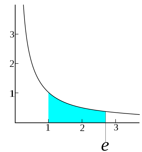
We can randomly generate numbers between 1 and $M$ (I will use $M=3$ here), order them, and estimate the integral for each random point. When the integral crosses from less than 1 to more than 1, stop:

from random import random
from math import e

N, Ni = 10*1000*1000, 0
ps = sorted([(1 + 3 * random(), random()) for _ in range(N)])
for i, p in enumerate(ps):
    if p[1] < 1 / p[0]: Ni += 1
    if (p[0]-1) * Ni / (i+1) > 1: break

print('actual:   %.5f' % e)
print('estimate: %.5f' % p[0])

Output:

actual:   2.71828
estimate: 2.71896

Here we also don't benefit from randomization: we can just start at 1, and increase by some small $\epsilon$ on each step, and stop if the integral is above 1, without using a list:

eps = 0.00000001
x = 1
integral = 0
while True:
    x += eps
    integral += eps * 1/x
    if integral > 1:
        break
print('actual:   %.5f' % e)
print('estimate: %.7f' % x)

Output:

actual:   2.7182818
estimate: 2.7182818

Estimating π

Estimating $\pi$ is easiest by using the definition of the area of a circle, $r^2 \pi$. We can randomly generate points $(x, y)$ in the square between $(-1, -1)$ and $(1, 1)$. The ratio of the number points such that $d^2 = x^2 + y^2 < r^2 = 1 $, ie. the points that fall within the circle with $r=1$, to the total number of points is equal to the ratio of the area of the circle $r^2 \pi$ to the area of the aquare $4r^2$:

from random import random
from math import pi

N = 10*1000*1000
Nc = sum([1 for _ in range(N) if random()**2 + random()**2 < 1])

print('actual:   %.5f' % pi)
print('estimate: %.5f' % (4 * Nc / N))

Output:

actual:   3.1412
estimate: 3.1416

As before, we can make it arbitrarily precise by using a grid:

eps = 0.0001
x = y = 0
Nc = N = 0
for _ in range(floor(1/eps)):
    for _ in range(floor(1/eps)):
        if x**2 + y**2 < 1: Nc += 1
        N += 1
        y += eps
    x += eps
    y = 0
print('actual:   %.5f' % pi)
print('estimate: %.5f' % (4 * Nc / N))

Output:

actual:   3.14159
estimate: 3.14199

Conclusion

Originally I wrote this article to demonstrate how very simple Monte Carlo simulations can be used to arrive at a reasonable estimate to these mathematical constants. This is true, but after I wrote the MC code, I realized that in most cases the approach can be re-formulated as a more efficient non-random grid search/integration. The grid methods are faster, use less (constant) storage, and the desired accuracy can be selected up front.