The german tank problem in World War II

Introduction

One of the challenges the Allies faced in World War II is knowing how many tanks the Germans had. Mathematically, the problem is the following: assume $N$ tanks are produced and numbered sequentially: $1, 2, 3... N$. $k < N$ tanks are destroyed, and their serial numbers are read off by soldiers and sent to a central intelligence agency. Based on these collected serial numbers, what is our best estimate for $N$? For the estimate to work, we assume that the destroyed tanks are a random sample from all the tanks, which may or may not be true in real life.

Per Wikipedia:

In the statistical theory of estimation, the German tank problem consists of estimating the maximum of a discrete uniform distribution from sampling without replacement. In simple terms, suppose there exists an unknown number of items which are sequentially numbered from 1 to N. A random sample of these items is taken and their sequence numbers observed; the problem is to estimate N from these observed numbers.

The problem can be approached using either frequentist inference or Bayesian inference, leading to different results. Estimating the population maximum based on a single sample yields divergent results, whereas estimation based on multiple samples is a practical estimation question whose answer is simple (especially in the frequentist setting) but not obvious (especially in the Bayesian setting).

The problem is named after its historical application by Allied forces in World War II to the estimation of the monthly rate of German tank production from very limited data. This exploited the manufacturing practice of assigning and attaching ascending sequences of serial numbers to tank components (chassis, gearbox, engine, wheels), with some of the tanks eventually being captured in battle by Allied forces.

Monte Carlo simulation

The solution is simple: we just have to order the serial numbers and compute the average gap between them. Then, we take the maximum and add the average gap. The intuition can be illustrated with a very small sample size. Imagine there are 100 tanks produced, and 3 are destroyed. If we randomly select 3 numbers, and order them, then the average of the smaller will be ~25, the middle one ~50, and the average of the bigger will be ~75, and the average gap will be ~25. The estimate for the number of tanks is $75+25=100$.

We can check our thinking with a simple Monte Carlo simulation:

num_tanks = 100
num_destroyed = 3
num_experiments = 1000*1000

destroyed_tanks = []
for _ in range(num_experiments):
    destroyed_tanks.append(sorted(sample(range(1, num_tanks+1), num_destroyed)))

print([mean([s[i] for s in destroyed_tanks]) for i in range(num_destroyed)])
estimate = mean([max(s) for s in destroyed_tanks]) + mean([(max(s)-min(s))/(len(s)-1) for s in destroyed_tanks])
print('Average estimate for num_tanks = %.2f' % estimate)

Prints something like:

[25.287, 50.517, 75.771]
Average estimate for num_tanks = 101.01

There is a small bug in our thinking. We expected the sorted averages to be [25, 50, 75], but they are approx. [25.25, 50.50, 75.75], the gap is 25.25 instead of 25, and the estimate is off by 1 (101 instead of 100). Why?

This is quite counter-intuitive (to me), it's because we're generating ints and not floats. Our intuition does work if we switch to floats:

num_tanks = 100
num_destroyed = 3
num_experiments = 1000*1000

destroyed_tanks = []
for _ in range(num_experiments):
    destroyed_tanks.append(sorted([uniform(1, num_tanks) for _ in range(num_destroyed)]))

print([mean([s[i] for s in destroyed_tanks]) for i in range(num_destroyed)])
estimate = mean([max(s) for s in destroyed_tanks]) + mean([(max(s)-min(s))/(len(s)-1) for s in destroyed_tanks])
print('Average estimate for num_tanks = %.2f' % estimate)

Prints something like:

[25.748, 50.498, 75.236]
Average estimate for num_tanks = 99.98

This is per our intuition, 50.5 is the midpoint between 1 and 100 (which is the interval we're uniformly sampling), and 25.75 is the midpoint between 1 and 50.5, and 75.25 is the midpoint between 50.5 and 100. Another way to see that the "quantization" by using integers matters is to think of the trivial example or 3 tanks and all 3 are destroyed: in this case the 3 numbers will [1, 2, 3], and clearly 1 is the not the midpoint between 1 and 2.

In any case, the actual formula for the least variance estimate for the number of tanks is:

$N = M + M/k - 1$

where $M$ is the maximum destroyed tank serial number and $k$ is the number of destroyed tanks. In code:

num_tanks = 100
num_destroyed = 3
num_experiments = 100*1000

destroyed_tanks = []
for _ in range(num_experiments):
    destroyed_tanks.append(sample(range(1, num_tanks+1), num_destroyed))

estimate = mean([max(s) + max(s)/len(s) - 1 for s in destroyed_tanks])
print('Average estimate for num_tanks = %.2f' % estimate)

Prints something like:

Average estimate for num_tanks = 100.01

Let's see how good this estimate is, and plot the standard deviation of for different $(N, k)$ combinations:

num_tanks = [100, 1000, 10*1000]
num_destroyed_ratio = [0.02, 0.05, 0.1, 0.2]
num_experiments = 10*1000

destroyed_tanks_dict = defaultdict(lambda: [])
for nt in num_tanks:
    for num_destroyed in [int(r*nt) for r in num_destroyed_ratio]:
        for _ in range(num_experiments):
            destroyed_tanks_dict[(nt, num_destroyed)].append(sample(range(1, nt+1), num_destroyed))

stdvs_dict = defaultdict(lambda: [])
for (nt, num_destroyed), destroyed_tanks in destroyed_tanks_dict.items():
    s = stdev([max(s) + max(s)/len(s) - 1 for s in destroyed_tanks])
    stdvs_dict[nt].append((num_destroyed, s))

plt.figure(figsize=(10,5))
plt.xlabel('k as a ratio of N')
plt.ylabel('stdev as ratio of N')
legends = []
for nt, stdvs in stdvs_dict.items():
    plt.plot([x[0]/nt for x in stdvs], [x[1]/nt for x in stdvs], marker='o')
    legends.append(f'N = {nt}')
plt.legend(legends)
plt.ylim((0, 0.5))
plt.show()

Shows:

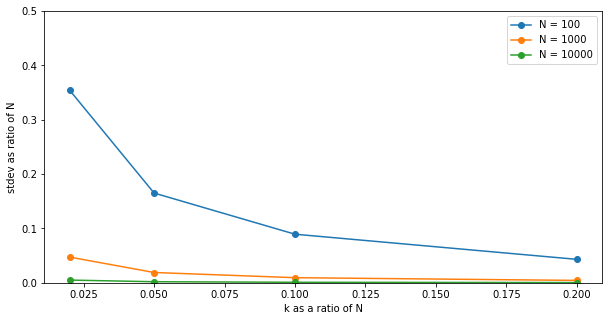
This shows that even at $N=1000$, if you are able to observe about 10% of serial numbers, you can expect to make a very good estimate, you will essentially be on target to within a few % when estimating $N$!

Conclusion

From the Wikipedia article:

According to conventional Allied intelligence estimates, the Germans were producing around 1,400 tanks a month between June 1940 and September 1942. Applying the formula below to the serial numbers of captured tanks, the number was calculated to be 246 a month. After the war, captured German production figures from the ministry of Albert Speer showed the actual number to be 245.