Introduction to Marketing Mix Modeling

Introduction

Imagine a Data Scientist asked to evaluate the effectiveness of an online marketing campaign. The golden standard in this situation is to scope the campaign as a Randomized Controlled Trial (RCT), also known as an A/B test:

1. Create a control and a test group which are statistically equal by selecting a large enough sample size, stratification, CUPED, etc; see my earlier post Five ways to reduce variance in A/B testing
2. Send the marketing campaign to the test group, and don't send it to control. Note that control may still receive other marketing campaign from the company, but not the one being tested.
3. Compare the Overall Evaluation Metric (OEM), usually sales between control and test, and report a % lift (and potentially extra sales).

This approach works great if we want to evaluate a single campaign, and if the Data Scientist is involved before the campaign runs, so she can re-scope it as an A/B test. But what if the question is about the overall effectiveness of marketing, not just online but also TV, radio, print, billboards, etc), and over a longer period of time. In this case, there are still two options for our Data Scientist:

1. For the online marketing component, the Data Scientist can recommend to scope it as a large, year-long test. This is likely to get strong pushback from the business, since not sending marketing to even 10% of customers (the control group) could negatively impact sales and cause the company to miss targets. Another difficulty may be technically implementing a "block" for the control group in a large, complex organization (with many business units and divisions spread across multiple countries).
2. The above approach of a large, year-long test doesn't work for offline marketing such as TV, radio, print, billboards, etc. because here randomization is not possible. We cannot tell people "you're in our control group, close your eyes and ears if you see or hear one of our ads". Also, in an RCT, the experimental units are not supposed to know which variant or group they are in, since that in itself may affect their behaviour and bias the results. The only way to test this would be if the Data Scientist would have access to a parallel universe where the company doesn't do any marketing for a year (but just this year), and then compare the OEM...

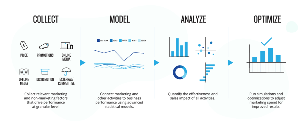
So, without access to parallel universes, what can the Data Scientist do? The industry answer is Marketing Mix Modeling (MMM):

Marketing mix modeling (MMM) is statistical analysis such as multivariate regressions on sales and marketing time series data to estimate the impact of various marketing tactics (marketing mix) on sales and then forecast the impact of future sets of tactics. It is often used to optimize advertising mix and promotional tactics with respect to sales revenue or profit.

The answer is to take ad spend data, promotions data, competitor ad spend data, competitor promotions, revenues, macro trends, etc. (everything we can get) and look for correlations, ie. build a model that explains historic sales resulting from a sum of:

• a seasonal baseline (the sales the model believes we would have without any marketing)
• marketing activities (ad campaigns, pricing, promotions)
• competitor effects (competitor's campaigns, pricings, promotions)
• macro influences (economy, exchange rates, Covid-19 lockdowns)

Some points worth noting:

• the most difficult task is likely to collect reliable and accurate input data, both about the company's own marketing and sales, as well as competitor's
• once some input data is available, we can use existing techniques and libraries (see below) to quickly get a model and answers to basic questions
• MMM is typically run using weekly level observations
• extra time and money should be spent on getting more and better quality data, not building more complicated models!
• if the model is built on low quality data then the results will be directional at best
• if our inputs are garbage, so will our conclusions — Garbage In, Garbage Out (GIGO)

The Marketer

From the perspective of the user — the Marketer — the objective is to understand how different marketing activities contribute to the outcome and then use that knowledge to optimize the allocation of marketing resources. MMM is particularly useful in multi-channel marketing strategies where various marketing tactics work in unison. These can range from traditional methods like TV, radio, print ads, to modern digital campaigns such as social media, email, and content marketing. By understanding the contribution of each of these elements, a marketer can make informed decisions on where to invest, what to optimize, and where to cut back.

The concept of MMM can be likened to a chef perfecting a recipe. Each marketing input represents an ingredient in the recipe. Just as a chef adjusts the ingredients to perfect the taste, a marketing analyst adjusts the marketing inputs to optimize sales. By evaluating historical data, MMM helps identify the effectiveness of each marketing input, providing insights on how to allocate budgets effectively and forecast future results.

Core MMM inputs

At the heart of a Marketing Mix Model are a variety of inputs that capture the full spectrum of marketing activities and external factors influencing sales or market share:

1. Marketing variables: These are the different marketing efforts put forth by a company across various channels. This can include spending on television ads, online marketing, radio, print, social media, direct mail, email campaigns, SEO, SEM, PR, promotions, sponsorships, and any other marketing channel the company is utilizing.

2. Sales data: This is the dependent variable that the model attempts to explain. It could be total sales, market share, or any other key performance indicator (KPI) that the organization uses to measure success.

3. Economic indicators: This includes factors like inflation rate, unemployment rate, GDP growth, and consumer sentiment, which can impact consumer buying behavior and in turn affect sales.

4. Competitive information: Details about competitor activities, such as their marketing spends, pricing changes, product launches, promotions, can influence your sales and should be included in the model.

5. Seasonality and trend variables: These capture predictable fluctuations in sales that are due to the time of year (like holiday seasons) or broader market trends.

6. Pricing and distribution information: Details on the pricing strategy and the distribution reach (number of stores, online presence, etc.) also play a critical role in influencing sales.

7. Product variables: Changes in product characteristics or the introduction of new products can impact sales. This can include changes in product features, packaging, branding, or the introduction of new SKUs.

These inputs help quantify the impact of each marketing activity on sales, allowing for more efficient allocation of marketing resources. By adjusting these inputs, companies can predict the potential impact of different marketing strategies on their overall sales performance.

Core MMM outputs

The Marketing Mix Model generates several important outputs that aid in understanding the performance and impact of marketing efforts:

1. Contribution by marketing input: This output quantifies the impact of each marketing channel on the target variable (e.g., sales or market share). This provides a breakdown of how much each marketing activity contributed to the total sales.

2. Return on Investment (ROI): ROI measures the profitability of each marketing activity by comparing the amount of profit generated to the cost of the activity. This allows marketers to understand which activities are most profitable.

3. Elasticities: This is a measure of how sensitive the target variable (e.g., sales) is to a change in a marketing input. For example, if the elasticity of sales with respect to TV advertising is 0.8, it means that a 1% increase in TV advertising spend would lead to a 0.8% increase in sales, all else being equal.

4. Baseline sales and incremental sales: Baseline sales are the sales that would have been achieved without any marketing activity, while incremental sales are the additional sales gained due to marketing efforts.

5. Synergies: Marketing activities often interact with each other, and the model can measure these synergies. For instance, a TV ad campaign may make an online campaign more effective, and the model would quantify this effect.

6. What-if scenarios/forecasts: Using the model, marketers can predict the impact of future marketing plans on sales. These scenarios can provide insights on how changes in the marketing mix can affect outcomes.

7. Optimal spending levels: Based on the ROI, the model can suggest the optimal level of spending for each marketing channel to maximize profit or sales.

These outputs enable marketers to evaluate their past marketing efforts and guide future investment decisions. They can also help identify areas of improvement, and optimize the marketing mix for better performance.

Google's MMM library

To make MMM more concrete, let's look at Google's opensource Lightweight MMM (LMMM) library. LMMM fits a bayesian additive model to the data in attempt to decompose the target variable (eg. sales) into a baseline (including a trend and seasonality) and the effect of marketing channels:

         $ kpi = \alpha + trend + seasonality + media\ channels + other\ factors $

Where $kpi$ is typically the volume or value of sales per time period, $\alpha$ is the model intercept, $trend$ is a flexible non-linear function that captures trends in the data, $seasonality$ is a sinusoidal function with configurable parameters that flexibly captures seasonal trends, $media\ channels$ is a matrix of different media channel activity (typically impressions or costs per time period) which receives transformations depending on the model used (see Media Saturation and Lagging section) and $other\ factors$ is a matrix of other factors that could influence sales. The full model is explained in the model documentation.

The below code runs LMMM with synthetic sample data (the code is from the LMMM Github repo):

import jax.numpy as jnp
import numpyro
from lightweight_mmm import lightweight_mmm
from lightweight_mmm import optimize_media
from lightweight_mmm import plot
from lightweight_mmm import preprocessing
from lightweight_mmm import utils

SEED = 105
data_size = 104 + 13
n_media_channels = 3
n_extra_features = 1
number_warmup=1000
number_samples=1000

media_data, extra_features, target, costs = utils.simulate_dummy_data(
    data_size=data_size,
    n_media_channels=n_media_channels,
    n_extra_features=n_extra_features)


split_point = data_size - 13
media_data_train = media_data[:split_point, ...]
media_data_test = media_data[split_point:, ...]
extra_features_train = extra_features[:split_point, ...]
extra_features_test = extra_features[split_point:, ...]
target_train = target[:split_point]

Here, we have 3 media channels, and 1 extra feature. An extra feature is just an extra timeseries that we think could be helpful for modeling, it could be something like inflation or a Covid-19 factor. Each of these is a timeseries of floats, with weekly or daily granularity. We can then fit the model:

media_scaler = preprocessing.CustomScaler(divide_operation=jnp.mean)
extra_features_scaler = preprocessing.CustomScaler(divide_operation=jnp.mean)
target_scaler = preprocessing.CustomScaler(divide_operation=jnp.mean)
cost_scaler = preprocessing.CustomScaler(divide_operation=jnp.mean, multiply_by=0.15)

media_data_train = media_scaler.fit_transform(media_data_train)
extra_features_train = extra_features_scaler.fit_transform(extra_features_train)
target_train = target_scaler.fit_transform(target_train)
costs = cost_scaler.fit_transform(costs)

mmm = lightweight_mmm.LightweightMMM(model_name="carryover")
mmm.fit(
    media=media_data_train,
    media_prior=costs,
    target=target_train,
    extra_features=extra_features_train,
    number_warmup=number_warmup,
    number_samples=number_samples,
    seed=SEED)

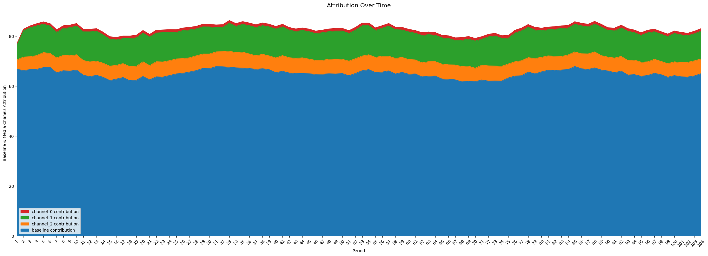
Now we can see how LMMM explains our target variable (eg. sales) using a generic baseline and the contributions from our marketing channel (3 channels in this example), ie. how sales is decomposed into a baseline, and 3 additional factors due to the 3 marketing channels:

media_contribution, roi_hat = mmm.get_posterior_metrics(
    target_scaler=target_scaler,
    cost_scaler=cost_scaler)
plot.plot_media_baseline_contribution_area_plot(media_mix_model=mmm,
    target_scaler=target_scaler,
    fig_size=(30,10))

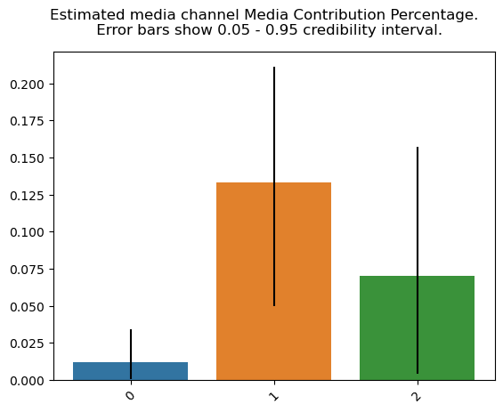
Next, what % of sales is coming from each marketing channel (unfortunately colors don't match with above chart):

plot.plot_bars_media_metrics(metric=media_contribution, metric_name="Media Contribution Percentage")

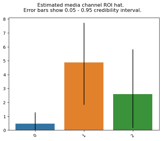
Each marketing channel's return on investment (ROI), ie. effectiveness:

plot.plot_bars_media_metrics(metric=roi_hat, metric_name="ROI hat")

Last, the response curves for the marketing channels, ie. how does their effectiveness vary with spend:

plot.plot_response_curves(media_mix_model=mmm, target_scaler=target_scaler, seed=SEED)

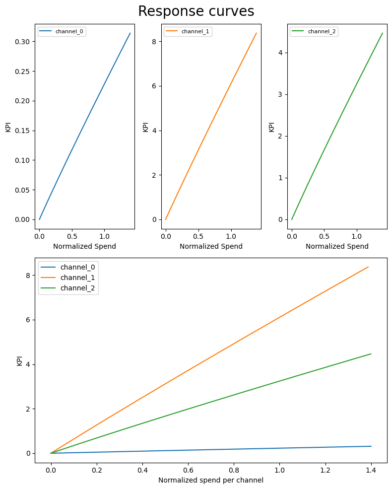
In this synthetic example, it's linear per channel, so every additional \$ spend marketing gets us the same additional \$ sales, although with a different ROI (slope) per channel.

Conclusion

Google's LMMM library does a lot more, both in terms of handling inputs, outputs and modeling, but for this introduction I will stop here. In the next post I will look at articles evaluating the accuracy of modeling advertising effectiveness.

Other good sources on MMM:

• Meta: Robyn MMM library
• Meta: Analyst's guide to MMM
• Google: Challenges And Opportunities In Media Mix Modeling (paper)
• TorwardsDataScience: How to Measure the Effectiveness of Advertising with Python & LMMM
• Recast blog (MMM vendor)
• Sellforte blog (MMM vendor)