Five ways to reduce variance in A/B testing
Marton Trencseni - Sun 19 September 2021 - ab-testing
Introduction
When performing A/B testing, we're measuring the mean of a metric (such as spend or conversion) on two distinct subsets, and then compare the means to each other. Because of the Central Limit Theorem, the measurement of the two means follows a normal distribution, as does the difference of the two (if A and B are normal, so is A - B).
Relevant Wikipedia articles:
Relevant Bytepawn articles:
Per the above, the variance of the lift (defined here as the difference) is $ s^2 = s_A^2 + s_B^2 $, where $s_A^2$ and $s_B^2$ are the variances of the A and B measurements, respectively, and $ s_i^2 = \frac{ \sigma^2 }{ N_i } $. So $ s^2 \approx \frac{\sigma^2}{N} $, where $\sigma^2$ is is the variance of the metric itself over the entire population.
I will use toy Monte Carlo simulations to illustrate 5 ways to reduce variance in A/B testing:
- increase sample size
- move towards an even split
- reduce variance in the metric definition
- stratification
- CUPED
The ipython notebook for this post is up on Github.
Increase sample size
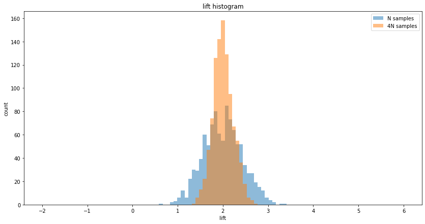
The simplest way to reduce variance is to collect more samples, if possible. For every 4x increase of $N$, we get a 2x decrement of $s$. In code:
def get_AB_samples(mu, sigma, treatment_lift, N):
    A = list(normal(loc=mu                 , scale=sigma, size=N))
    B = list(normal(loc=mu + treatment_lift, scale=sigma, size=N))
    return A, B

N = 1000
N_multiplier = 4
mu = 100
sigma = 10
treatment_lift = 2
num_simulations = 1000

print('Simulating %s A/B tests, true treatment lift is %d...' % (num_simulations, treatment_lift))

n1_lifts, n4_lifts = [], []
for i in range(num_simulations):
    print('%d/%d' % (i, num_simulations), end='\r')
    A, B = get_AB_samples(mu, sigma, treatment_lift, N)
    n1_lifts.append(lift(A, B))
    A, B = get_AB_samples(mu, sigma, treatment_lift, N_multiplier*N)
    n4_lifts.append(lift(A, B))

print('N samples  A/B testing, mean lift = %.2f, variance of lift = %.2f' % (mean(n1_lifts), cov(n1_lifts)))
print('4N samples A/B testing, mean lift = %.2f, variance of lift = %.2f' % (mean(n4_lifts), cov(n4_lifts)))
print('Raio of lift variance = %.2f (expected = %.2f)' % (cov(n4_lifts)/cov(n1_lifts), 1/N_multiplier))

bins = linspace(-2, 6, 100)
plt.figure(figsize=(14, 7))
plt.hist(n1_lifts, bins, alpha=0.5, label='N samples')
plt.hist(n4_lifts, bins, alpha=0.5, label=f'{N_multiplier}N samples')
plt.xlabel('lift')
plt.ylabel('count')
plt.legend(loc='upper right')
plt.title('lift histogram')
plt.show()
Prints:
Simulating 1000 A/B tests, true treatment lift is 2...
N samples  A/B testing, mean lift = 2.00, variance of lift = 0.18
4N samples A/B testing, mean lift = 2.01, variance of lift = 0.05
Raio of lift variance = 0.26 (expected = 0.25)
Note: in real life, collecting more samples is not always possible, since the amount of samples may be limited, or there may be a time limit by which we want to conclude the experiment. Also, in many situations, the relationship of the length of time $t$ that the experiment runs and sample size $N$ is sub-linear, because over time users tend to return. In other words, if we run an experiment for 2 weeks, and get $2N$ users, running it for another 2 weeks will probably yield less than $2N$ additional users.
Move towards an even split
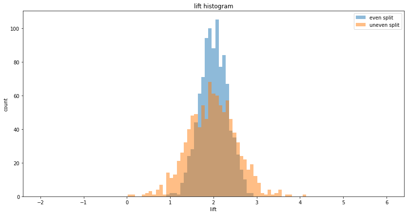
If we have $N$ samples available to use for A/B testing, one question is, what percent to put into A (control) and what percent to put into B (treatment). Almost always there are risk-management concerns, but it's worth knowing that in terms of the best lift measurement (lowest variance), the most optimal split is the even split of 50%-50%, and a 20%-80% split is better than a 10%-90%. We can see this with simple math. Suppose our $N$ total samples are split into $pN$ and $(1-p)N$ for A and B variants, then the variance is:
$ s^2 = \frac{ \sigma^2 }{ pN } + \frac{ \sigma^2 }{ (1-p)N } = \frac{ \sigma^2 }{ N } ( \frac{1}{p} + \frac{1}{1-p} ) $.
So, $ s^2(p) = C ( \frac{1}{p} + \frac{1}{1-p} ) $, which has a minimum at $p=\frac{1}{2}$:
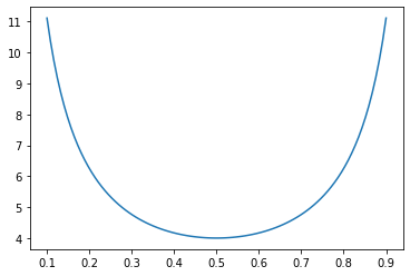
The more the split is away from even, the higher the variance compared to the optimal case:
def get_AB_samples(mu, sigma, treatment_lift, N_A, N_B):
    A = list(normal(loc=mu                 , scale=sigma, size=N_A))
    B = list(normal(loc=mu + treatment_lift, scale=sigma, size=N_B))
    return A, B

def expected_ratio(p, q):
    top = 1/p + 1/(1-p)
    bot = 1/q + 1/(1-q)
    return top/bot

N = 4000
mu = 100
sigma = 10
treatment_lift = 2
even_ratio = 0.5
uneven_ratio = 0.9
num_simulations = 1000

print('Simulating %s A/B tests, true treatment lift is %d...' % (num_simulations, treatment_lift))

even_lifts, uneven_lifts = [], []
for i in range(num_simulations):
    print('%d/%d' % (i, num_simulations), end='\r')
    A, B = get_AB_samples(mu, sigma, treatment_lift, int(N*even_ratio), int(N*(1-even_ratio)))
    even_lifts.append(lift(A, B))
    A, B = get_AB_samples(mu, sigma, treatment_lift, int(N*uneven_ratio), int(N*(1-uneven_ratio)))
    uneven_lifts.append(lift(A, B))

print('Even split   A/B testing, mean lift = %.2f, variance of lift = %.2f' % (mean(even_lifts),   cov(even_lifts)))
print('Uneven split A/B testing, mean lift = %.2f, variance of lift = %.2f' % (mean(uneven_lifts), cov(uneven_lifts)))
print('Raio of lift variance = %.2f (expected = %.2f)' % ((cov(even_lifts)/cov(uneven_lifts)), expected_ratio(even_ratio, uneven_ratio)))
Prints:
Simulating 1000 A/B tests, true treatment lift is 2...
Even split   A/B testing, mean lift = 1.98, variance of lift = 0.10
Uneven split A/B testing, mean lift = 1.98, variance of lift = 0.29
Raio of lift variance = 0.36 (expected = 0.36)
Reduce variance in the metric definition
In the equation $ s^2 = \frac{ \sigma^2 }{ N } $, the previous two methods were increasing the sample size $N$ to reduce $s^2$. Another way to reduce $s^2$ is to reduce the variance $ \sigma^2 $ of the underlying metric itself. I will mention two approaches here:
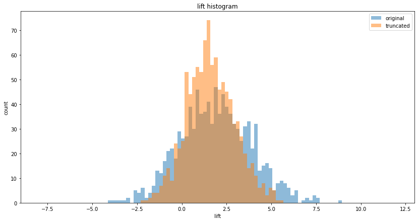
1. Winsorizing, ie. cutting or normalizing outliers. For example, if the underlying metric is spend per head, there may be outliers, such as high-value B2B customers among the overall population of B2C customers, or bots appearing to spend a lot of time on a site compared to real users. If we cut-off these values at some $\sigma$ (technically, we can either discard these values or set them to the highest acceptable value), we will get a better measurement of our "real" population:
def get_AB_samples(scale, treatment_lift, N):
    A = list(exponential(scale=scale                 , size=N))
    B = list(exponential(scale=scale + treatment_lift, size=N))
    # add outliers
    for i in range(int(N*0.001)):
        A.append(random()*scale*100)
        B.append(random()*scale*100 + treatment_lift)
    return A, B

N = 10*1000
scale = 100
treatment_lift = 2
num_simulations = 1000

orig_lifts, trunc_lifts = [], []
for i in range(num_simulations):
    print('%d/%d' % (i, num_simulations), end='\r')
    A, B = get_AB_samples(scale, treatment_lift, N)
    orig_lifts.append(lift(A, B))
    A, B = [x for x in A if x < 5*scale], [x for x in B if x < 5*scale]
    trunc_lifts.append(lift(A, B))
Another method is to measure the median instead of the mean. Note that with these approaches we are changing the definition of the metric itself. So, for example, Finance's "spend per head" definition may no longer match the winsorized or median-based definition of the experimentation framework!
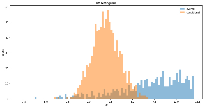
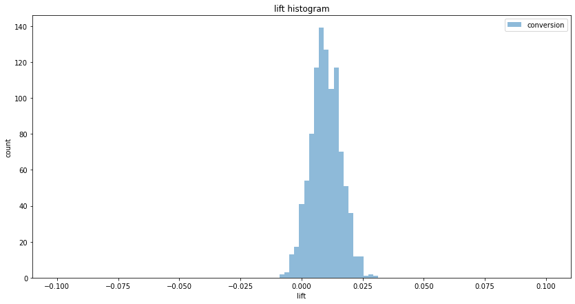
2. Measuring a metric further down the funnel. Suppose we are measuring a metric such as spend per head. We can split this metric into two parts:
(spend per head, overall) = (ratio of users who spend more than 0, conversion) x (spend per head of those who spend more than zero, conditional)
In real-life, the ratio is usually low, less than 10%. In such cases, measuring the two terms (the conversion and the conditional) separately yields lower variance:
def get_AB_samples(p, p_lift, mu, sigma, treatment_lift, N_A, N_B):
    A = list(normal(loc=mu                 , scale=sigma, size=N_A))
    B = list(normal(loc=mu + treatment_lift, scale=sigma, size=N_B))
    A = [x if random() < p        else 0 for x in A]
    B = [x if random() < p+p_lift else 0 for x in B]
    return A, B

N = 10*1000
p = 0.1
p_lift = 0.01
mu = 100
sigma = 25
treatment_lift = 2
num_simulations = 1000

print('Simulating %s A/B tests, true treatment lift is %d...' % (num_simulations, treatment_lift))

cont_lifts, cond_lifts, conv_lifts = [], [], []
for i in range(num_simulations):
    print('%d/%d' % (i, num_simulations), end='\r')
    A, B = get_AB_samples(p, p_lift, mu, sigma, treatment_lift, int(N/2), int(N/2))
    cont_lifts.append(lift(A, B)/p)
    A_, B_ = [x for x in A if x > 0], [x for x in B if x > 0]
    cond_lifts.append(lift(A_, B_))
    A_, B_ = [1 if x > 0 else 0 for x in A], [1 if x > 0 else 0 for x in B]
    conv_lifts.append(lift(A_, B_))

bins = linspace(-8, 12, 100)
plt.figure(figsize=(14, 7))
plt.hist(cont_lifts, bins, alpha=0.5, label='overall')
plt.hist(cond_lifts, bins, alpha=0.5, label='conditional')
plt.xlabel('lift')
plt.ylabel('count')
plt.legend(loc='upper right')
plt.title('lift histogram')
plt.show()

bins = linspace(-0.1, 0.1, 100)
plt.figure(figsize=(14, 7))
plt.hist(conv_lifts, bins, alpha=0.5, label='conversion')
plt.xlabel('lift')
plt.ylabel('count')
plt.legend(loc='upper right')
plt.title('lift histogram')
plt.show()
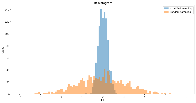
Stratification
Stratification lowers variance by making sure that each sub-population is sampled according to its split in the overall population. As a toy example, assume there are two sub-populations, M and F, with different distributions. For simplicity let's assume that the population is exactly 50% M and 50% F. In an A/B test, if we randomly sample the overall population and assign them to A and B, we will on approximately get 50% Ms and 50% Fs in both A and B, but not exactly. This small difference will impact our measurement variance. However, if we make sure that both A and B have exactly 50% Ms and 50% Fs, the variance of the measurement is decreased:
def get_AB_samples_str(
    pop1_mu, pop1_sigma,
    pop2_mu, pop2_sigma,
    pop1_ratio,
    treatment_lift,
    N,
):
    A =  list(normal(loc=pop1_mu, scale=pop1_sigma, size=int(N*pop1_ratio)))
    A += list(normal(loc=pop2_mu, scale=pop2_sigma, size=int(N*(1-pop1_ratio))))
    B =  list(normal(loc=pop1_mu + treatment_lift, scale=pop1_sigma, size=int(N*pop1_ratio)))
    B += list(normal(loc=pop2_mu + treatment_lift, scale=pop2_sigma, size=int(N*(1-pop1_ratio))))
    return A, B

def get_AB_samples_rnd(
    pop1_mu, pop1_sigma,
    pop2_mu, pop2_sigma,
    pop1_ratio,
    treatment_lift,
    N,
):
    A = []
    for _ in range(N):
        if random() < pop1_ratio:
            A.append(normal(loc=pop1_mu, scale=pop1_sigma))
        else:
            A.append(normal(loc=pop2_mu, scale=pop2_sigma))
    B = []
    for _ in range(N):
        if random() < pop1_ratio:
            B.append(normal(loc=pop1_mu + treatment_lift, scale=pop1_sigma))
        else:
            B.append(normal(loc=pop2_mu + treatment_lift, scale=pop2_sigma))
    return A, B


N = 4000
pop1_ratio = 0.5
pop1_mu = 100
pop2_mu = 200
pop1_sigma = pop2_sigma = 10
treatment_lift = 2
num_simulations = 1000

print('Simulating %s A/B tests, true treatment lift is %d...' % (num_simulations, treatment_lift))

str_lifts, rnd_lifts = [], []
for i in range(num_simulations):
    print('%d/%d' % (i, num_simulations), end='\r')
    A, B = get_AB_samples_str(pop1_mu, pop1_sigma, pop2_mu, pop2_sigma, pop1_ratio, treatment_lift, N)
    str_lifts.append(lift(A, B))
    A, B = get_AB_samples_rnd(pop1_mu, pop1_sigma, pop2_mu, pop2_sigma, pop1_ratio, treatment_lift, N)
    rnd_lifts.append(lift(A, B))

print('Stratified sampling   A/B testing, mean lift = %.2f, variance of lift = %.2f' % (mean(str_lifts), cov(str_lifts)))
print('Random sampling       A/B testing, mean lift = %.2f, variance of lift = %.2f' % (mean(rnd_lifts), cov(rnd_lifts)))
print('Raio of lift variance = %.2f' % (cov(str_lifts)/cov(rnd_lifts)))
Prints:
Simulating 1000 A/B tests, true treatment lift is 2...
Stratified sampling   A/B testing, mean lift = 2.01, variance of lift = 0.05
Random sampling       A/B testing, mean lift = 1.97, variance of lift = 1.28
Raio of lift variance = 0.04
If we cannot control the sampling of the population, we can also re-weigh samples after data collection is over. Stratification and CUPED are closely related, check section 3.1 and 3.3 of the CUPED paper.
CUPED
CUPED is a way to reduce variance in A/B testing if the past historic values of the metric are correlated wit the current values we measure in the experiment. In other words, CUPED works if eg. high spenders before the experiment also tend to be high spenders during the experiment, and the same for low spenders. I have written four articles on CUPED, so I will just link to those:
- Reducing variance in A/B testing with CUPED
- Reducing variance in conversion A/B testing with CUPED
- A/A testing and false positives with CUPED
- Correlations, seasonality, lift and CUPED
Conclusion
The post used toy examples to show some of the fundamental methods and levers to reduce variance in experiments. It's worth noting that I used Monte Carlo simulations over many experiments (typically 1,000) to show the decrease in variance, by visualizing the spread of the lift histogram. The point is, in one specific experiment evaluation, the decrease is not visible, since one measurement does not have variance-of-lift by itself (it's just one specific lift we measure). The rewards of lower variance in A/B testing are reaped in the long term, by having more accurate measurements, making better decisions and releasing better products more quickly.