Introductory investigations into the stability of stock price volatility
Marton Trencseni - Sun 25 February 2024 - Finance
Introduction
As part of my private investor journey, I invest a significant fraction of my reading time into finance books. For example, I found the following generic interest books insightful:
- Warren Buffett: Berkshire Hathaway Letters to Shareholders
- Charlie Munger: The Complete Investor
- Soros on Soros: Staying Ahead of the Curve
- Trading at the Speed of Light
- In Pursuit of the Perfect Portfolio
As I was reading the last book on the list (In Pursuit..), and was amused that most discussions start at Markowitz portfolio theory and CAPM, which I've studied at University. Now, 25 years later, with the power of easy to use Python packages and freely available high-quality stock datasets, the assumptions of these models can be tested by anybody, at home, on their laptop --- e.g. me!
First, what is Markowitz portfolio theory, also knows as Modern Portfolio Theory? From Wikipedia:
Modern portfolio theory (MPT), or mean-variance analysis, is a mathematical framework for assembling a portfolio of assets such that the expected return is maximized for a given level of risk. It is a formalization and extension of diversification in investing, the idea that owning different kinds of financial assets is less risky than owning only one type. Its key insight is that an asset's risk and return should not be assessed by itself, but by how it contributes to a portfolio's overall risk and return. The variance of return (or its transformation, the standard deviation) is used as a measure of risk, because it is tractable when assets are combined into portfolios.[1] Often, the historical variance and covariance of returns is used as a proxy for the forward-looking versions of these quantities, but other, more sophisticated methods are available. Economist Harry Markowitz introduced MPT in a 1952 essay, for which he was later awarded a Nobel Memorial Prize in Economic Sciences; see Markowitz model.
Closely related is the Capital Asset Pricing Model (CAPM), introduced by Sharpe. From Wikipedia:
The model takes into account the asset's sensitivity to non-diversifiable risk (also known as systematic risk or market risk), often represented by the quantity beta (β) in the financial industry, as well as the expected return of the market and the expected return of a theoretical risk-free asset. CAPM assumes a particular form of utility functions (in which only first and second moments matter, that is risk is measured by variance, for example a quadratic utility) or alternatively asset returns whose probability distributions are completely described by the first two moments (for example, the normal distribution) and zero transaction costs (necessary for diversification to get rid of all idiosyncratic risk). Under these conditions, CAPM shows that the cost of equity capital is determined only by beta. Despite its failing numerous empirical tests, and the existence of more modern approaches to asset pricing and portfolio selection (such as arbitrage pricing theory and Merton's portfolio problem), the CAPM still remains popular due to its simplicity and utility in a variety of situations.
The basic ideas are:
- each stock or security is assumed to have a expected return and variance (volatility)
- a rational investor prefers, for a fixed variance, maximum expected return, or, for fixed expected return, minimal variance
- the securities have non-zero covariance
- securities can be combined into a portfolio, which has a combined expected return and variance
- these optimal (return, variance) points form the efficient frontier, rational investors pick stocks and portfolios here
- by picking the right stocks in the right proportions, overall portfolio variance can be reduced (individual variances cancel out to some degree)
- so the points on the efficient frontier are in practice portfolios, not individual stocks
- there is a zero variance, usually non-zero security on the market, eg. US government bonds
- by putting the zero variance security into the mix, the efficient frontier always becomes a line
One of the aspects of the theory that intrigues me is: is the volatility of a security stable and knowable? In other words, if I measure the variance of a security's return in the past, can I reasonably assume it will be the same looking ahead, eg. in the next year?
The code for this article is on Github.
Note: in this post I use the terms "standard deviation", "variance" and "volatility" in an imprecise manner. Standard deviation is the square root of variance, and volatility is standard deviation of log returns.
Volatility of tech stocks
Here I will start to investigate this basic question using simple checks on a few stocks that I personally invest in: Apple, Microsoft, Tesla, Meta, Google. This is straightforward thanks to the wonderful yfinance Yahoo Finance API package. Downloading the daily stats is as simple as:
tickers = ['AAPL', 'MSFT', 'TSLA', 'META', 'GOOG']
df = yf.download(tickers, '2014-01-01', '2023-12-31')
Then, compute and plot daily changes:
df_diffs = df['Close'].diff()
df_diffs.plot()
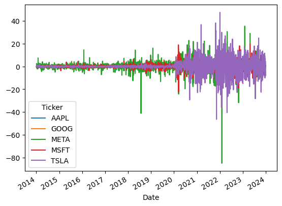
This immediately shows that Meta had some big swings, but Tesla seems to have the most daily volatility. Also, these stocks started to become much more volatile around 2020, at least in absolute USD daily changes.
In general, we expect standard deviation to be related to stock price, ie. a stock with a higher USD price will have higher daily USD variations. This can be checked visually. First, download the 2023 data:
url = 'https://en.m.wikipedia.org/wiki/Nasdaq-100'
df_nasdaq100 = pd.read_html(url, attrs={'id': "constituents"}, index_col='Ticker')[0]
tickers = list(df_nasdaq100.index)
df_nasdaq_100 = yf.download(tickers, '2023-01-01', '2023-12-31')
Now, compare the 2023 USD mean stock price to the daily USD standard deviation in price:
means  = [df_nasdaq_100['Adj Close'].mean()[t] for t in tickers]
sigmas = [df_nasdaq_100['Adj Close'].std()[t]  for t in tickers]
plt.scatter(means, sigmas, marker='.')
plt.xlim([0, 500])
plt.ylim([0, 100])
plt.title('2023 Nasdaq Top 100 daily adj closing price')
plt.xlabel('mean of daily adj closing price')
plt.ylabel('stdev of daily adj closing price')
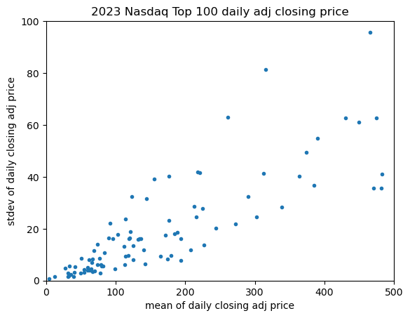
The linear correlation is nicely visible. A similar check can be made for the variance of the daily USD return:
df_diffs = df_nasdaq_100['Close'].diff()
means = {t:df_nasdaq_100['Close'].mean()[t] for t in tickers}
volatilities = {t:stdev([x for x in list(df_diffs[t]) if x == x]) for t in tickers}
means = [x[1] for x in sorted(means.items())]
volatilities = [x[1] for x in sorted(volatilities.items())]
plt.scatter(means, volatilities, marker='.')
plt.xlim([0, 500])
plt.ylim([0, 15])
plt.title('2023 Nasdaq Top 100 daily adj closing price')
plt.xlabel('mean of daily adj closing price')
plt.ylabel('stdev of daily change in adj close')
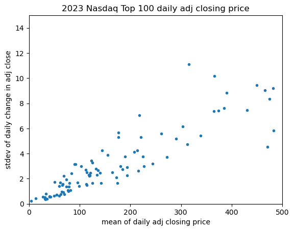
The linear correlation is again nicely visible.
Next, I want to compute from daily changes annual statistics, and compare them against each other, year after year. For this I wrote a short helper function:
def show_volatilities(df, relative=False, price_col='Close'):
if relative:
df_diffs = df[price_col].pct_change()
else:
df_diffs = df[price_col].diff()
tickers = list(df_diffs.columns)
df_diffs['Year'] = df_diffs.index.year
df_diffs.head()
sigmas = defaultdict(lambda: [])
years = sorted(list(set(list(df_diffs['Year']))))
for t in tickers:
for y in years:
li = list(df_diffs.loc[df_diffs['Year'] == y][t])
# get rid of nans:
li = [x for x in li if x == x]
s = stdev(li)
sigmas[t].append(s)
legend = []
errors = defaultdict()
for t, series in sigmas.items():
plt.plot(years, series, marker='o')
legend.append(t)
estimate = mean(series[:-1])
actual = series[-1]
abs_error = abs(estimate - actual)
rel_error = abs_error / actual
mul = 100 if relative else 1
errors[t] = (actual*mul, estimate*mul, abs_error*mul, rel_error)
for t, e in errors.items():
if relative:
print(f'The actual 2023 stdev for {t} was {e[0]:.2f}%, the historic estimate was {e[1]:.2f}%, an absolute error of {e[2]:.2f}% (relative {100*e[3]:.1f}%)')
else:
print(f'The actual 2023 stdev for {t} was ${e[0]:.2f}, the historic estimate was ${e[1]:.2f}, an absolute error of ${e[2]:.2f} (relative {100*e[3]:.1f}%)')
print()
plt.legend(legend)
plt.xlabel('year')
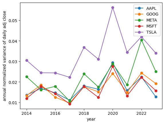
plt.ylabel(f'annual{" normalized " if relative else " "}variance of daily {price_col.lower()}')
The function also computer how much of an error we would make if we compute the average volatility from the historic timeseries (2014-2022), and then compares it to the 2023 actual volatility.
Running it for the tech stocks:
tickers = ['AAPL', 'MSFT', 'TSLA', 'META', 'GOOG']
df_tech = yf.download(tickers, '2014-01-01', '2023-12-31')
show_volatilities(df_tech, relative=False))
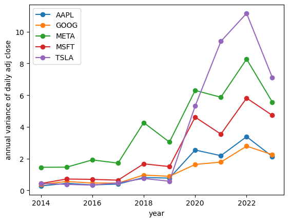
The actual 2023 stdev for AAPL was $2.14, the historic estimate was $1.28, an absolute error of $0.87 (relative 40.4%)
The actual 2023 stdev for GOOG was $2.25, the historic estimate was $1.10, an absolute error of $1.15 (relative 51.2%)
The actual 2023 stdev for META was $5.57, the historic estimate was $3.82, an absolute error of $1.76 (relative 31.5%)
The actual 2023 stdev for MSFT was $4.76, the historic estimate was $2.27, an absolute error of $2.49 (relative 52.2%)
The actual 2023 stdev for TSLA was $7.11, the historic estimate was $3.20, an absolute error of $3.91 (relative 55.0%)
This shows that there is significant variation from one year to the next.
Next, I wondered whether it would make more sense to look at the daily variation as percent changes. After all, if a $100 stock goes to $102, that's a 2% return, much better than if a $1000 stock goes to $1002, only a 0.2% return. In real life, investor care about percent returns, not absolute USD price changes. This can be triggered by the relative=True flag in the show_volatilities() functions:
show_volatilities(df_tech, relative=True)
The actual 2023 stdev for AAPL was 1.28%, the historic estimate was 1.76%, an absolute error of 0.48% (relative 37.9%)
The actual 2023 stdev for GOOG was 1.93%, the historic estimate was 1.67%, an absolute error of 0.25% (relative 13.0%)
The actual 2023 stdev for META was 2.51%, the historic estimate was 2.19%, an absolute error of 0.33% (relative 12.9%)
The actual 2023 stdev for MSFT was 1.58%, the historic estimate was 1.63%, an absolute error of 0.05% (relative 3.3%)
The actual 2023 stdev for TSLA was 3.40%, the historic estimate was 3.36%, an absolute error of 0.05% (relative 1.3%)
In this picture, the prediction errors are quite small, and interestingly Tesla has the lowest error of 1.3%, although this feels like a lucky coincidence.
Perhaps trying to predict volatility using 9 years is too long. How about if we always try to predict the next year's volatility using the previous year, ie. year-over-year? What is the annual error of our prediction? To check this, a minor variation of the previous helper function:
def show_yoy_volatilities(df, relative=False, price_col='Adj Close'):
    if relative:
        df_diffs = df[price_col].pct_change()
    else:
        df_diffs = df[price_col].diff()
    tickers = list(df_diffs.columns)
    df_diffs['Year'] = df_diffs.index.year
    df_diffs.head()
    sigmas = defaultdict(lambda: [])
    years = sorted(list(set(list(df_diffs['Year']))))
    for t in tickers:
        for y in years:
            li = list(df_diffs.loc[df_diffs['Year'] == y][t])
            # get rid of nans:
            li = [x for x in li if x == x]
            s = stdev(li)
            sigmas[t].append(s)
    legend = []
    errors = defaultdict(lambda: [])
    for t, series in sigmas.items():
        for i in range(len(series)-1):
            cy = series[i+1] # current year
            py = series[i]   # previous year
            abs_error = abs(cy - py)
            rel_error = abs_error / cy
            errors[t].append(rel_error)
    legend = []
    for t, e in errors.items():
        legend.append(t)
        plt.plot(years[1:], e, marker='o')
    print()
    plt.legend(legend)
    plt.xlabel('year')
    plt.ylabel(f'yoy annual{" normalized " if relative else " "}variance of daily {price_col.lower()}')
Checking the year-over-year volatility change in absolute daily prices for our tech stocks:
show_yoy_volatilities(df_tech, relative=False)
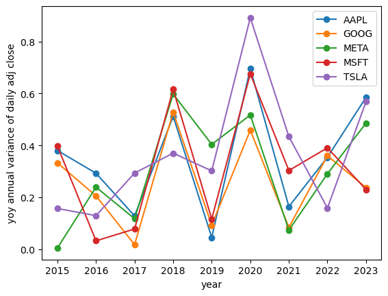
Checking the year-over-year volatility change of daily percentage returns of our tech stocks:
show_yoy_volatilities(df_tech, relative=True)
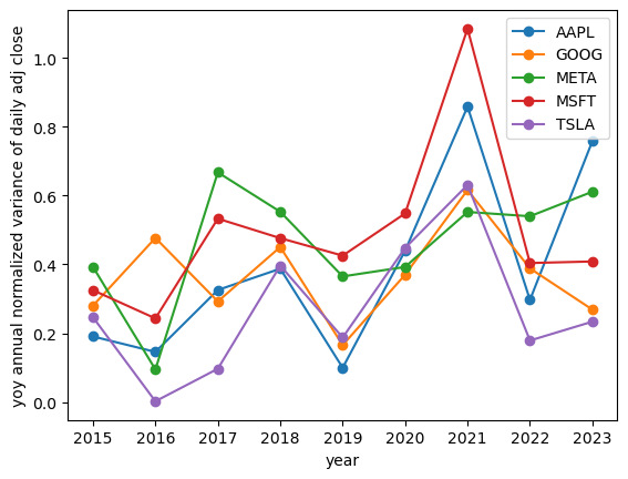
The plots indicate that with this method we would make 20-50-100% errors.
Volatility of global indexes
The next thing I wondered is whether index stocks' volatility is more predictable? I check 5 global indexes:
GSPC: S&P500DJI: Dow JonesIXIC: Nasdaq CompositeGDAXI: DAX (40 german bluechips)N225: Nikkei 225 (Tokyo stock market index)
# https://finance.yahoo.com/world-indices/
tickers = ['^GSPC', '^DJI', '^IXIC', '^GDAXI', '^N225']
df_indices = yf.download(tickers, '2014-01-01', '2023-12-31')
show_volatilities(df_indices, relative=False)
show_volatilities(df_indices, relative=True)
show_yoy_volatilities(df_indices, relative=False)
show_yoy_volatilities(df_indices, relative=True)
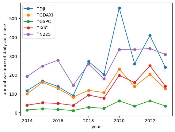
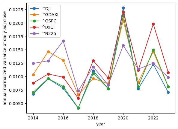
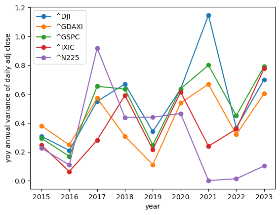
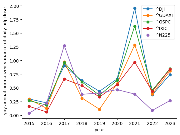
Interestingly, the index volatility does appear to be smaller than that of individual stocks; but year over year it's shows the same lack of stability.
Conclusion
These simple checks are not enough to draw far reaching conclusions, but it seems it's not trivial to estimate the volatility of securities. I plan to run further, more systematic checks in upcoming posts.