Modern Portfolio Theory I: Random portfolio coverage in log volatility—return space
Marton Trencseni - Sun 01 December 2024 - Finance
Introduction
Understanding the interplay between risk and return is a core area of research in Econometrics and portfolio management. Harry Markowitz's pioneering work on Modern Portfolio Theory (MPT) introduced the concept of the efficient frontier — a set of optimal portfolios offering the highest expected return for a defined level of risk. Building upon this foundation, the Capital Asset Pricing Model (CAPM) further explores the relationship between systematic risk and expected return, providing a cornerstone for asset pricing and portfolio selection.
This article begins to explore these foundational theories by simulating random portfolios within the log volatility—return space: we use Monte Carlo methods to generate random portfolios and visualize their coverage in terms of volatility and return.
The artice is organized as follows:
- Data download: Downloading 2023 daily closing prices for the stocks constituting the Nasdaq-100.
- Log returns: Transforming price data into log returns to normalize the returns and make them additive over time — a common practice in quantitative finance.
- Random portfolios: Creating a series of random portfolios using different Monte Carlo randomization schemes.
- Log volatility and return computation: Calculating the expected return and volatility for each portfolio to understand their placement in volatility—return space.
- Visualization: Plotting the portfolios and their convex hulls to observe the spread and to identify any emergent patterns or the presence of an efficient frontier.
By simulating portfolios randomly, we aim to uncover insights into how portfolios might naturally distribute themselves in the volatility—return space without active optimization, and how this depends on the number of non-zero stocks in the portfolio. The code is up on Github.
Data download
This step is straightforward with the yfinance library:
# download 2023 Nasdaq-100 daily closing prices
url = 'https://en.m.wikipedia.org/wiki/Nasdaq-100'
df_nasdaq100 = pd.read_html(url, attrs={'id': "constituents"}, index_col='Symbol')[0]
tickers = list(df_nasdaq100.index)
df_nasdaq_100 = yf.download(tickers, '2023-01-01', '2023-12-31')
The result is a dataframe with $S=100$ stocks and their closing prices for the $T=250$ trading days of 2023.
Returns and log returns
Why are we using log returns in portfolio theory? The answer is simple: we want to be able to compute the mean and volatility (standard deviation) of our time window's daily returns. However, regular returns don't work for this: a simple example is, if on day 1 the return is $1.5$ (+50%), and the next day it's $0.5$ (-50%), the mean of $1.5$ and $0.5$ is $1$, but the return is actually $1.5 \cdot 0.5 = 0.75$ (-25%)! Doing linear statistics on returns doesn't work, because returns are meant to be multiplied, not added. However, if we take their logarithm, then we can add them, because multiplication in linear space is addition in log space: $log(ab)=log(a)+log(b)$. In other words, if we have a series of log returns, and their mean is $0$, it means the original returns multiply to produce $1$.
Converting to log returns is straightforward with numpy:
# log returns
df_logr = np.log(df_nasdaq_100['Adj Close']).diff()[1:]
Note that the dataframe containing the log returns has 1 less row than trading days, so $T'=249$ for 2023. Once we have log returns, the regular returns are:
# regular returns
df_r = np.exp(df_logr)
Portfolio returns: it's worth pointing out that daily portfolio returns have to be calculated using the weighted sum of daily regular returns of the stocks, and then the logarithm is taken to get the portfolio's log return. Using the weighted sum of daily log returns of stocks is not equivalent and leads to incorrect results!
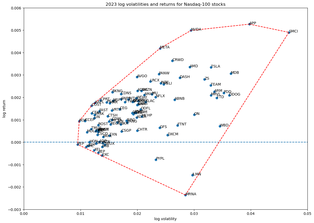
The log volatility—return space of the 100 Nasdaq-100 stocks is shown below, with their convex hull shown in red:
Random portfolios
Creating random portfolios and computing their volatility and returns is simple: each portfolio is a unit weight vector of the $S=100$ stocks (summing to 1). On each trading day, the portfolio's log return is the logarithm of the scalar product of the portfolio weight vector and the daily bare stock returns. The result is daily log returns for the portfolio.
# makes a vector of n-dimensions, sets weight at positions set_weights, with values weight_values
def set_weights(n, indexes, weight_values):
    ws = np.zeros(n)
    for index, i in enumerate(indexes):
        ws[i] = weight_values[index]
    return ws

# make a random portfolio of length num_tickers, with all but portfolio_size tickers zeroed out
def random_portfolio(num_tickers, portfolio_size=2):
    indexes = np.random.choice(np.arange(num_tickers), size=portfolio_size, replace=False)
    weight_values = unit_random(portfolio_size)
    portfolio_weights = list(set_weights(num_tickers, indexes, weight_values))
    return portfolio_weights

# make many random_portfolios
def random_portfolios(num_tickers, portfolio_size=2, num_simulations=1_000):
    return [random_portfolio(num_tickers, portfolio_size) for _ in range(num_simulations)]

# given per ticker returns in ar for a trading window, compute and return the
# volatility and return for a portfolio in this trading window
def portfolio_return(ar, portfolio_weights):
    num_tickers = len(ar[0])
    portfolio_returns = []
    for day in range(len(ar)):
        daily_return = sum([portfolio_weights[i]*ar[day][i] for i in range(num_tickers)])
        portfolio_return = np.log(daily_return) # portfolio log return for given day
        portfolio_returns.append(portfolio_return)
    std = np.sqrt(np.var(portfolio_returns))
    avg = np.mean(portfolio_returns)
    return std, avg

# compute and return the volatility and return for many portfolios
def portfolio_returns(df, portfolios):
    ar = np.nan_to_num(df.to_numpy(), nan=1)
    xs, ys = [], []
    for i, portfolio in enumerate(portfolios):
        print(f'Computing return for portfolio {i+1:,} of {len(portfolios):,}      ', end='\r')
        std, avg = portfolio_return(ar, portfolio)
        xs.append(std)
        ys.append(avg)
    return xs, ys

# make num_simulations random portfolios, each with all portfolio_size tickers zeroes out, compute and return the volatily and return for each
def simulate_portfolios(df, portfolio_size=2, num_simulations=10_000):
    num_tickers = len(df.columns.values)
    ps = random_portfolios(num_tickers, portfolio_size, num_simulations)
    return portfolio_returns(df, ps)
The function random_portfolio(num_tickers, portfolio_size) creates a random vector of num_tickers elements, all set to 0, with the exception of portfolio_size random elements, which are set to random numbers that sum to 1. Invoking this function yields results such as:
random_portfolio(3, 1)
> [0.0, 1.0, 0.0]

random_portfolio(3, 2)
> [0.0, 0.32276196035546617, 0.6772380396445339]

random_portfolio(3, 2)
> [0.5515248563282706, 0.0, 0.44847514367172936]
random_portfolio() internally first decides which elements to set in the portfolio vector:
indexes = np.random.choice(np.arange(num_tickers), size=portfolio_size, replace=False)
Then it uses the function unit_random() to get a dense vector of random numbers summing to 1:
weight_values = unit_random(portfolio_size)
Then it sets the appropriate values in the sparse portfolio vector.
Randomization strategies
The code listing above did not show the implementation of unit_random(), which we will discuss here. Although it seems like a trivial function to write, it turns out there is beauty and non-trivial implications of how we implement it. The naive way to implement would be:
# makes a random unit vector of n-dimensions
def unit_random_simple(n):
    ws = np.random.random(n)
    return ws / np.sum(ws)
The core issue with this version is that at high dimensions, which is what we have with num_tickers=100 and high portfolio_size values, this naive way of solving this problem leads to a random portfolio where most weights are around $1/k$, where $k$ is the number of set non-zero weights (portfolio_size in the code). The reason is simple: each element of ws will be between $0$ and $1$, at large $k$ their sum will be around $k/2$, and then each is divided by that, so mostly they will fall between $0$ and $2/k$. We can see this in action:
unit_random_simple(10)
> [0.07747502, 0.09647462, 0.06158791, 0.14403998, 0.16212218,
       0.05422107, 0.17737698, 0.0689759, 0.13414295, 0.02358338]
This will "never" return a portfolio where $1$ out of $10$ weights is $0.9$ and the remaining $9$ add up to $0.1$, it's just too unlikely, and at higher dimensions it gets even worse! The problem is that this means that as we increase our portfolio size, we don't really explore the full possibility of random portfolios, we just explore a small space around the uniform balanced portfolio consisting of all $1/k$ weights.
We need a better randomization technique, one that returns all sorts of uneven portfolio combinations as well. To address this I have written a total of 3 versions of unit_random():
# makes a random unit vector of n-dimensions
def unit_random_simple(n):
    ws = np.random.random(n)
    return ws / np.sum(ws)

def unit_random_dirichlet(n, bias=1):
    return np.random.dirichlet(np.ones(n)*bias, size=1)[0]

def unit_random_angle_projection(n):
    ws = np.tan(np.random.rand(n) * np.pi/2) # unit cirlce projected out to x-axis
    return ws / np.sum(ws)
The Dirichlet version was suggested by a Stackoverflow post, whose points I will not repeat here. unit_random_angle_projection() is my own version, which takes a random angle in the lower right quadrant of the unit circle centered in $(0, 1)$, and projects it out to the x-axis to get a random number between 0 and $\infty$. This will favor small values, but can return arbitrarily large ones as well. I found this version to produce the best random portfolios in terms of coverage in log volatility—return space. Here is an example:
unit_random_angle_projection(10)
> [0.08540684, 0.01795899, 0.01126532, 0.06939637, 0.03126648,
       0.01231148, 0.69112335, 0.04299283, 0.00796563, 0.03031272]
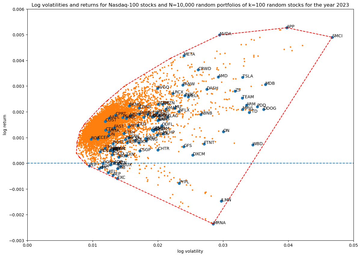
For comparison, here are $N=10,000$ random portfolios at $k=100$ portfolio size (all stocks used in the portfolio) with unit_random_angle_projection():
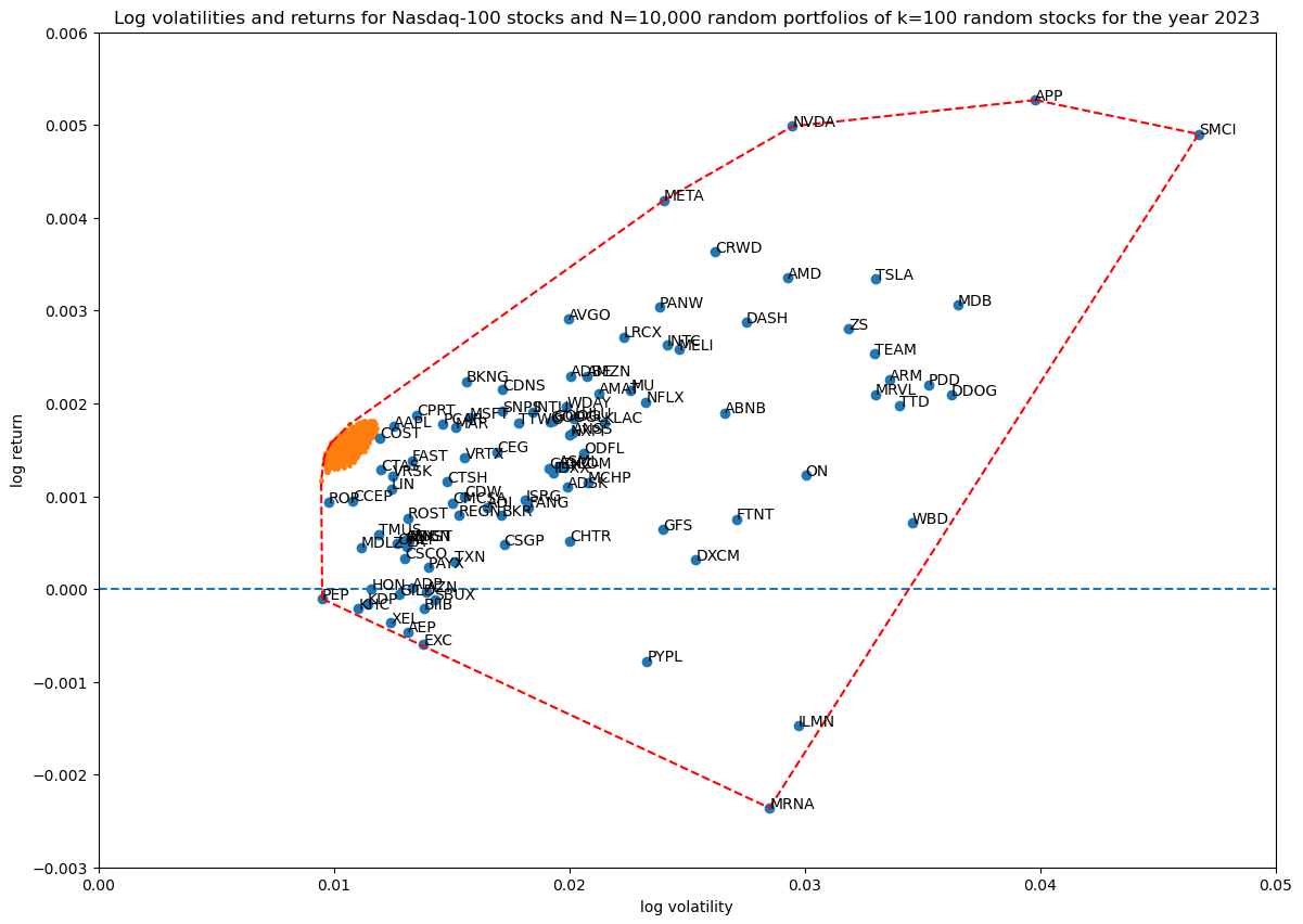
The same, but using unit_random_simple(). We can see all the portfolios are bunching up in one area in log volatility—return space:
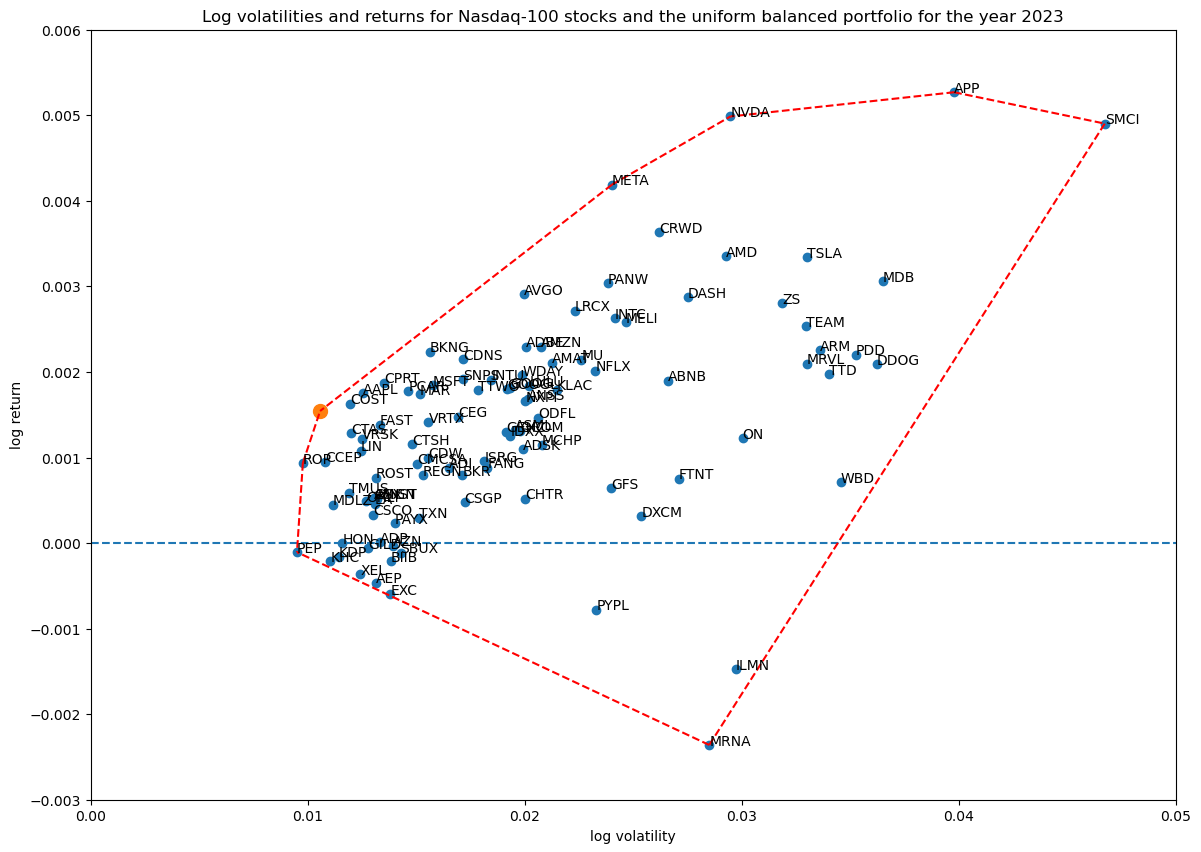
For reference, here is the uniform balanced portfolio, where each weight is $1/S=0.01$. Clearly the points above are spreading around this one portfolio:
In the rest of the article, all Monte Carlo simulations use unit_random_angle_projection(), unless called out specifically.
Coverage in log volatility—return space as a function of random portfolios
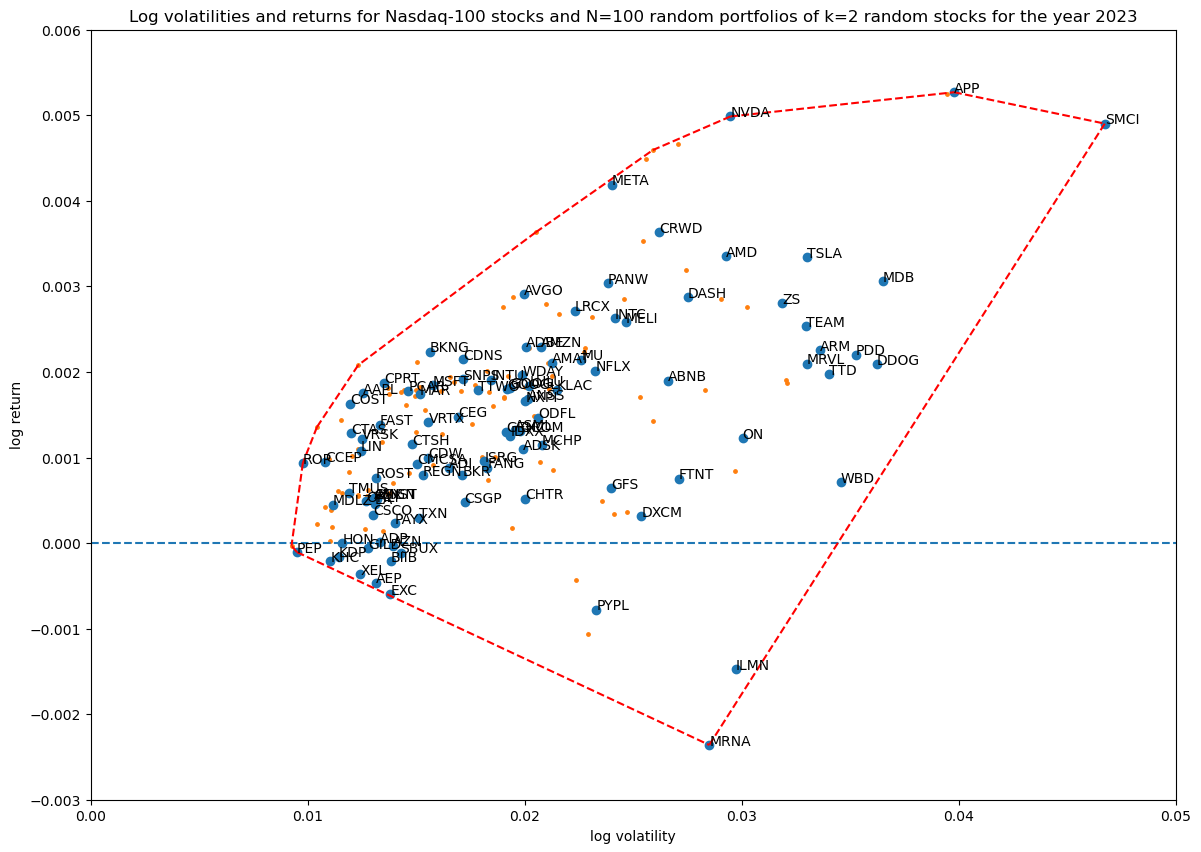
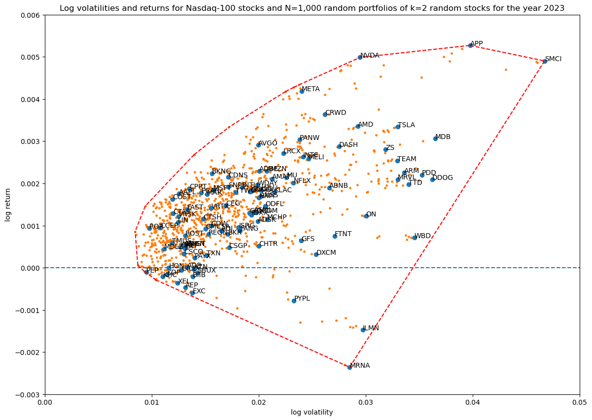
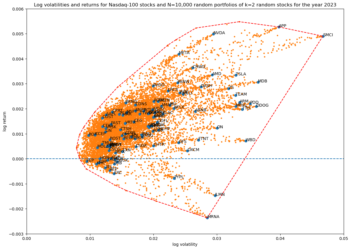
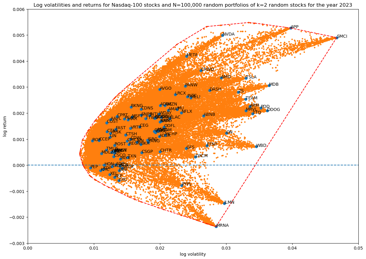
First I wanted to see how many Monte Carlo runs of random portfolios are needed to get good enough coverage of the portion of the log volatility—return space that is reachable at a certain portfolio size:
portfolio_size = 2
for num_simulations in [100, 1_000, 10_000, 100_000]:
    title = f'...'
    portfolios = simulate_portfolios(df_r, portfolio_size, num_simulations)
    hulls[portfolio_size][num_simulations] = plot_portfolios(bare, portfolios, title)
This results in the following diagrams:
Showing the convex hulls (which also contains the original stocks) of all the runs in one plot for comparison:
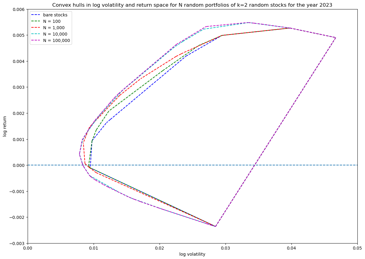
Based on this $N=10\,000$ simulations are enough to get good coverage.
Coverage in log volatility—return space as a function of portfolio size
Next, let's see how increasing the number of non-zero stocks in the portfolio weight vector increases coverage in log volatility—return space:
num_simulations = 10_000
for portfolio_size in [3, 5, 10, 50, 100]:
    title = f'...'
    portfolios = simulate_portfolios(df_r, portfolio_size, num_simulations)
    hulls[portfolio_size][num_simulations] = plot_portfolios(bare, portfolios, title)
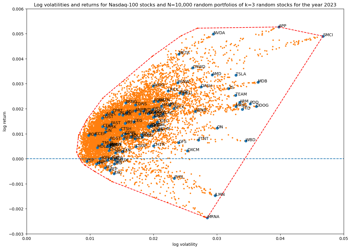
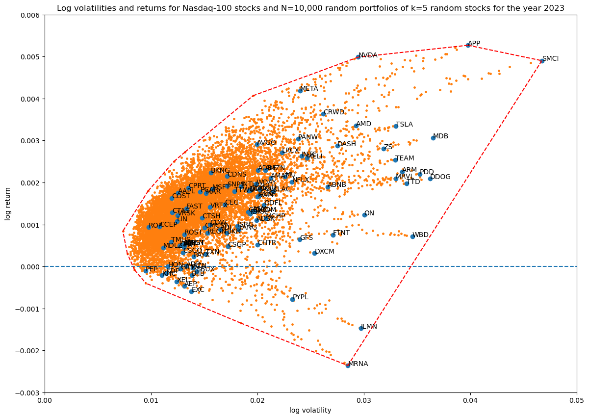
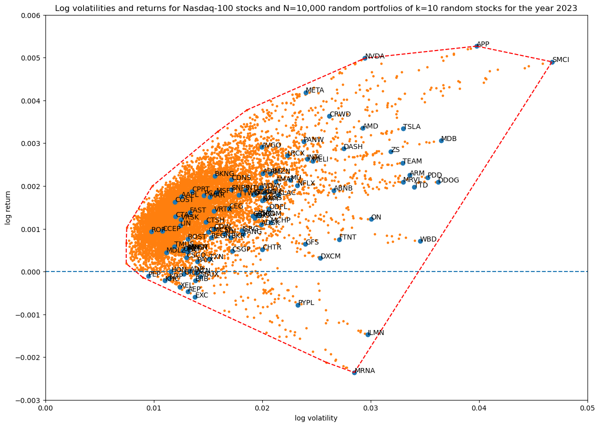


Showing the convex hulls (which also contains the original stocks) of all the runs in one plot for comparison:
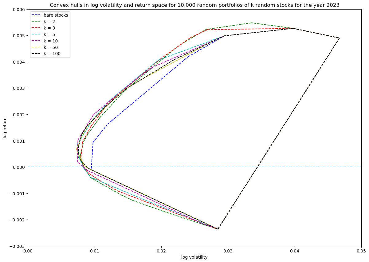
It's quite interesting that coverage does not seem to go up considerably, in fact the high volatility—high return region is easier explored with a smaller portfolio. This of course makes sense, since less stocks will be more risky (higher volatility), and the payout for risk is a potentially higher return.
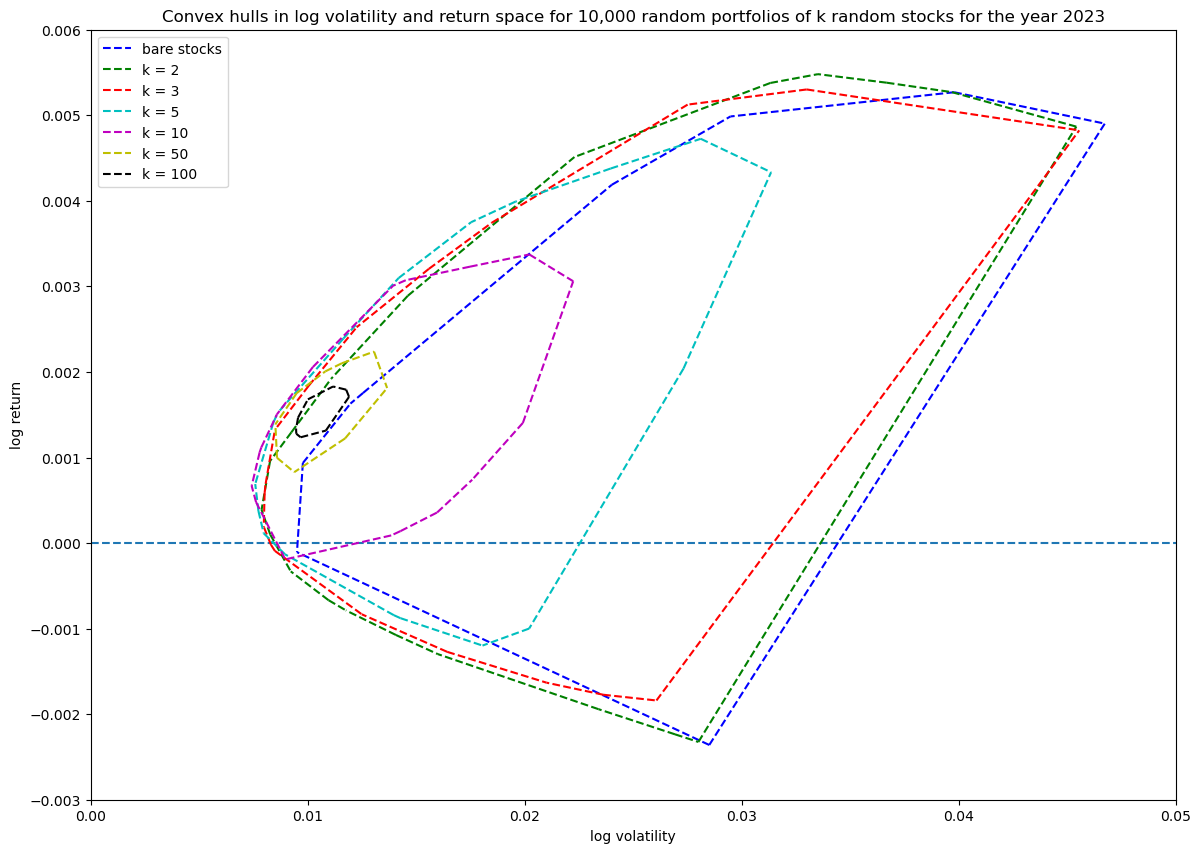
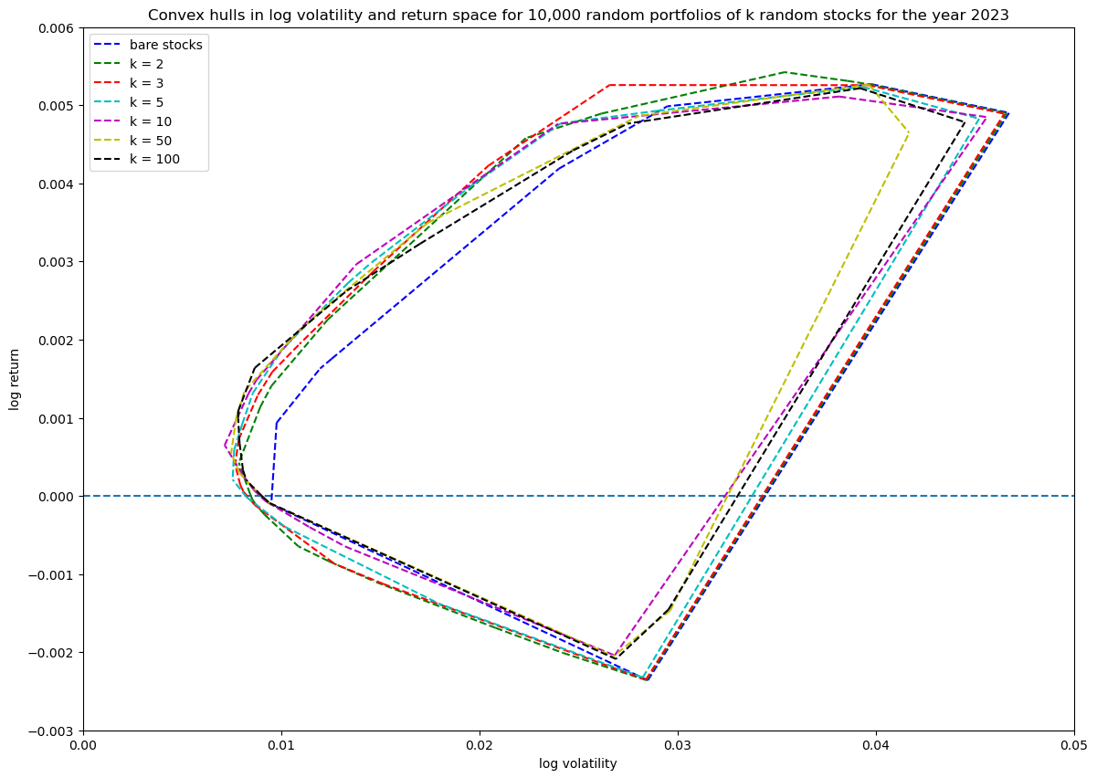
For completeness, I will show the same convex hull series plot but, without including the original bare stocks, both computed with the unit_random_simple() function and the unit_random_angle_projection() function. It shows beautifully how the explored region gets smaller with the first function as portfolio size increases and the weight vector gets closer to the uniformly balanced portfolio weight vector.
Progression of convex hull (without including bare stocks in the hull) for unit_random_simple():
Progression of convex hull (without including bare stocks in the hull) for unit_random_angle_projection():
Discussion
The visualizations from our simulations offer insightful observations into how random portfolios behave within the log volatility-return space, and how these behaviors relate to the principles of Modern Portfolio Theory (MPT) and the Capital Asset Pricing Model (CAPM):
1. Diversification and risk: As the portfolio size increases, the dispersion of portfolio returns and volatilities decreases. Portfolios with more stocks tend to cluster closer together in the risk-return space. This aligns with MPT's assertion that diversification reduces unsystematic risk. By holding a larger number of assets, the unique risks of individual stocks tend to cancel out, resulting in a portfolio that more closely reflects the overall market risk and return.
2. Hints of an efficient frontier: The convex hulls of the random portfolios outline a boundary in the log volatility—return space, resembling the efficient frontier described in MPT. While our random portfolios are not optimized, the outer edge of their distribution suggests the limits of achievable returns for given levels of risk. This highlights that, through optimization, it's possible to construct portfolios that lie on this efficient frontier, maximizing expected return for a given level of risk, or minimizing risk for a given level or return.
3. Random portfolios vs. optimal portfolios: Randomly generated portfolios scatter throughout the feasible region but do not necessarily occupy the optimal positions on the efficient frontier. This underscores the importance of strategic portfolio construction. MPT emphasizes that without optimization, portfolios are unlikely to be efficient.
Next steps
This was a lengthy first step to explore the econometrics of stocks and other investing instruments. I plan to look at many more aspects in following posts, for example:
- how to convert the log space back to regular annual metrics and how to interpret them
- interpretations and alternatives to standard deviation based volatility
- examination of the validity of implicit assumptions made, such as normal or log-normal distributions
- introducing the risk-free asset and the efficient frontier of CAPM
- examining the covariance matrix of stocks and factor investing