Probabilistic spin glass - Part II
Marton Trencseni - Sat 18 December 2021 - Physics
Introduction
This is a continuation of the previous article on probabilistic spin glasses, with improvements to the simulation code and improved entropy computation. The ipython notebook is up on Github.
Symmetry
In the previous article I generated probabilistic spin glasses such as neighbouring spins are aligned with probability $p$. The code used started in the top left corner, first generated the first spin with probability $p_0$, and then used $P(s=1 | n=1) = p$ to generate the spins in the first row. The first element in the second row is again trivial to generate using $p$, then each spin has 2 neighbours, so I derived the conditional formula for 2 neighbours. To be sure the construction is correct, I ran Monte Carlo simulations: I generated a large number of spin glasses, and made sure that neighbouring spins are aligned with probability $p$.
However, the construction still has a shortcoming. We would expect spin glasses that are "the same" to be generated with equal probability. Ie. if X and Y are spin glasses and X is an up-down or left-right mirror or for square grids a 90° rotation (or an arbitrary combination of the previous 3) of Y, then X and Y are really "the same", and should be generated with the same probability in a Monte Carlo ensemble.
Let's check this for the code from the previous article. Let's generate a large number of grids, and count the frequencies:
num_simulations = 10*1000*1000
rows, cols, p0, p, d = 2, 2, 0.5, 0.9, 4
frequencies = Counter()
for i in range(num_simulations):
    if i % 100 == 0:
        pct = int((i / num_simulations) * 10000) / 100
        print(f'Computing grid probabilities for the {rows}x{cols} spin glass, progress {pct}% ', end='\r')
        sys.stdout.flush()
    grid = create_grid(rows, cols, p0, p)
    frequencies[json.dumps(grid.tolist())] += 1

fig, axs = plt.subplots(d, d, figsize=(10, 10))
for i, (grid, f) in enumerate(frequencies.most_common()):
    ax = axs[i // d, i % d]
    ax.imshow(np.array(json.loads(grid)), cmap='hot', vmin=0, vmax=1)
    ax.axes.get_xaxis().set_visible(False)
    ax.axes.get_yaxis().set_visible(False)
    ax.set_title(f'p=%0.4f' % (f/num_simulations))
plt.show()
Yields:
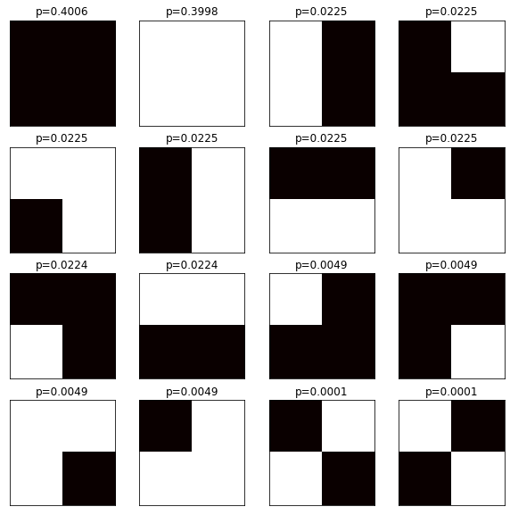
The symmetry does not hold! The first grid in the 2nd row and the first grid in the last row are the same after a left-right flip, but their probabilities are not the same! There are two ways to fix the construction:
- When generating the grid, randomly pick the starting point (top or bottom, left or right) and randomly pick the starting direction (horizontal or vertical). Implementing it yields hard to read code.
- Generate the grid using the simple code from the previous article, then randomly apply one of the 8 symmetry transformations.
Let's do the second:
def create_grid(rows, cols, p0, p):
    # ...
    # code from previous article generates grid
    # ...
    # make the ensemble symmetric
    if random() < 0.5:
        grid = np.fliplr(grid)
    if random() < 0.5:
        grid = np.flipud(grid)
    if rows == cols and random() < 0.5:
        grid = np.rot90(grid)
    return grid.astype(int)
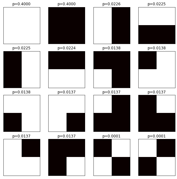
After this, the probabilities for grids in the same symmetry groups are equal:
Probabilities instead of Statistics
In the above example, I generated 10,000,000 grids to get good sample size. But this is not really required. For a $ N \times K $ spin glass, there are $ 2^{N \times K} $ up-down spin combinations. We can turn the construction process on its head: instead of using the probabilities to generate random grids, we can just enumerate all possible grids, and compute the probability of generating that. The basic logic is very similar to the Monte Carlo simulation:
def spin_glass_probability_inner(grid, p0, p):
    rows, cols = grid.shape
    cp2 = calculate_conditional_probs_for_1(p0, p)
    grid_probability = 1
    # first element
    grid_probability *= cp(grid[0, 0], p0)
    # first row
    for j in range(1, cols):
        grid_probability *= cp(grid[0, j-1] == grid[0, j], p)
    # remaining rows
    for i in range(1, rows):
        grid_probability *= cp(grid[i-1, 0] == grid[i, 0], p)
        for j in range(1, cols):
            grid_probability *= cp(grid[i, j], cp2['%d%d' % (grid[i-1, j], grid[i, j-1])])
    return grid_probability
However, this has the same symmetry problem, let's fix that:
def spin_glass_probability(grid, p0, p):
    grid_probability = 0
    # create all possible symmetry transformations of grid
    # all combinations of left-right, up-down mirroring and 90 degree rotation
    # total of 2^3 = 8 transformations, including identity, ie. no transformation
    # the symmetric probability of the grid is the average probability
    grid_probability += spin_glass_probability_inner(grid, p0, p)
    grid_probability += spin_glass_probability_inner(np.fliplr(grid), p0, p)
    grid_probability += spin_glass_probability_inner(np.flipud(grid), p0, p)
    grid_probability += spin_glass_probability_inner(np.fliplr(np.flipud(grid)), p0, p)
    normalization = 4
    if rows == cols:
        grid_probability += spin_glass_probability_inner(np.rot90(grid), p0, p)
        grid_probability += spin_glass_probability_inner(np.fliplr(np.rot90(grid)), p0, p)
        grid_probability += spin_glass_probability_inner(np.flipud(np.rot90(grid)), p0, p)
        grid_probability += spin_glass_probability_inner(np.fliplr(np.flipud(np.rot90(grid))), p0, p)
        normalization += 4
    return grid_probability / normalization
    #
    # without honoring symmetries:
    # return spin_glass_probability_inner(grid, p0, p)
We can now compare this to the Monte Carlo simulation to verify that we compute the same probabilities for each $2 \times 2$ grid:
rows, cols, p0, p, d = 2, 2, 0.5, 0.9, 4
probabilities = Counter()
for li in list(itertools.product([0, 1], repeat=rows*cols)):
    grid = np.asarray(li).reshape(rows, cols).astype(int)
    grid_probability = spin_glass_probability(grid, p0, p)
    probabilities[json.dumps(grid.tolist())] = grid_probability

fig, axs = plt.subplots(d, d, figsize=(10, 10))
for i, (grid, grid_probability) in enumerate(probabilities.most_common()):
    ax = axs[i // d, i % d]
    ax.imshow(np.array(json.loads(grid)), cmap='hot', vmin=0, vmax=1)
    ax.axes.get_xaxis().set_visible(False)
    ax.axes.get_yaxis().set_visible(False)
    ax.set_title(f'p=%0.4f' % grid_probability)
plt.show()
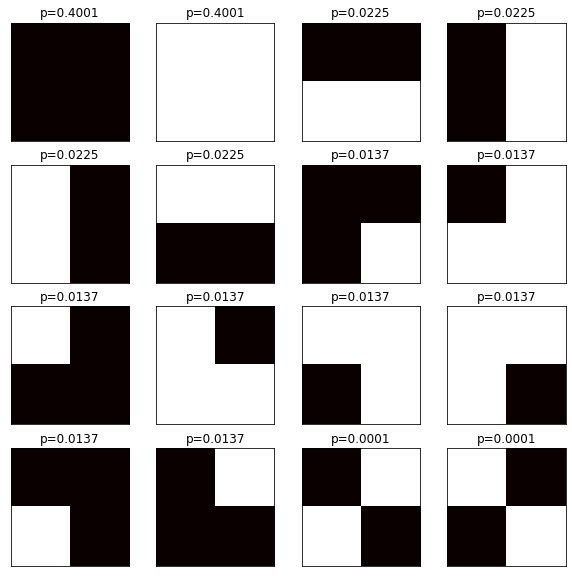
With this approach we don't waste CPU time generating 10,000,000 samples. The Monte Carlo version took 203 seconds, this took just a few miliseconds!
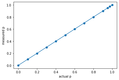
There is still value in the Monte Carlo method, since computing all $ 2^{N \times K} $ combinations is not feasable for large spins, eg. a $ 100 \times 100 $ spin glass has $2^{10,000}$ spin combinations. By the time we go through that, the Sun has exploded and the Universe has ended. Here the MC method's importance sampling is still preferable. Let's use MC to draw the calibration curve for a $ 100 \times 100 $ grid using 100 samples, to make sure the generated grids obey the desired probabilities:
# consistency check
num_simulations = 100
rows, cols, p0 = 100, 100, 0.5
ps = []
for p in [ZERO, 0.1, 0.2, 0.3, 0.4, 0.5, 0.6, 0.7, 0.8, 0.9, ONE]:
    same, total = 0, 0
    for _ in range(num_simulations):
        grid = create_grid(rows, cols, p0, p)
        for i in range(0, rows-1):
            for j in range(0, cols-1):
                if grid[i, j] == grid[i+1, j]:
                    same += 1
                if grid[i, j] == grid[i, j+1]:
                    same += 1
                total += 2
    measured_p = same/total
    ps.append((p, measured_p))

plt.plot([x[0] for x in ps], [x[1] for x in ps], marker='o')
plt.xlabel('actual p')
plt.ylabel('measured p')
Yields:
Entropy
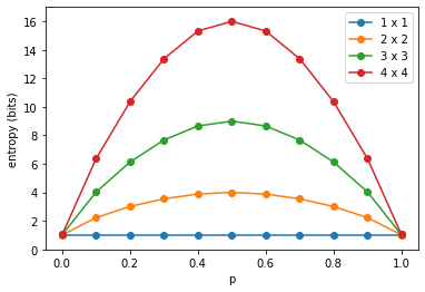
Next, let's see how entropy varies with grid size for square grids. Since we can directly compute the probability of each grid, we enumerate the grids, get the probabilities, and use the standard formula for entropy:
def spin_glass_entropy(rows, cols, p0, p, base=2):
    entropy = 0
    for i, li in enumerate(list(itertools.product([0, 1], repeat=rows*cols))):
        grid = np.asarray(li).reshape(rows, cols).astype(int)
        grid_probability = spin_glass_probability(grid, p0, p)
        entropy -= grid_probability * log(grid_probability, base)
    return entropy

grid_entropies = []
for n in [1, 2, 3, 4]:
    for p in [ZERO, 0.1, 0.2, 0.3, 0.4, 0.5, 0.6, 0.7, 0.8, 0.9, ONE]:
        h = spin_glass_entropy(rows=n, cols=n, p0=p0, p=p)
        grid_entropies.append((n, p, h))

for n in sorted(list(set([x[0] for x in grid_entropies]))):
    xs = [x[1] for x in grid_entropies if x[0] == n]
    ys = [x[2] for x in grid_entropies if x[0] == n]
    plt.plot(xs, ys, marker='o')
plt.xlabel('p')
plt.ylabel('entropy (bits)')
plt.legend(sorted(list(set(['%d x %d' % (x[0], x[0]) for x in grid_entropies]))))
plt.ylim((0, 17))
Yields:
We can plot the same another way, drawing lines for indentical proabilities $p$:
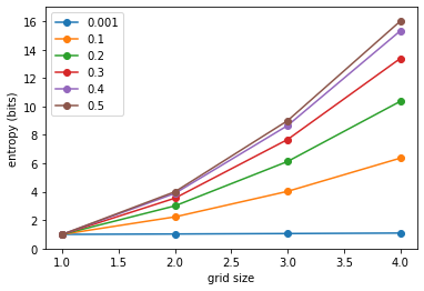
For a given grid size, the entropy $H(p)$ is concave. For a given probability $p$, the entropy $H(N)$ is convex and scales like $O(N^2)$ for a $N \times N$ spin glass (for $p=0.5$, entropy is exactly $H(N)=N^2$).
Conclusion
The main lesson here was that it's not always necessary to perform Monte Carlo simulations. Sometimes it's possible to enumerate all possibilities with the appropriate proabilities. When computing the entropy, this is preferred, since importance sampling does not necessarily yield a good approximation of entropy.