Random Walks and the Dickey-Fuller Test - Part II
Marton Trencseni - Sat 26 April 2025 - Finance
Introduction
In the last post, Random Walks and the Dickey-Fuller Test, we laid the groundwork for unit-root testing. We reviewed why the weak-form Efficient-Market Hypothesis implies stock prices should follow a random walk, introduced the Dickey–Fuller (DF) framework, and derived the core AR(1) formulation:
$ \Delta y_t \;=\; \gamma\,y_{t-1} + \varepsilon_t, \qquad H_0:\gamma = 0. $
We then walked through a pure NumPy implementation of the DF statistic, used Monte Carlo simulation to generate finite-sample critical-value tables, and visualised the non-standard DF distribution. Finally, five synthetic series—white noise, sine wave, random walk, linear-trend-plus-noise, and mean-reverting AR(1)—showed how the test behaves in practice and matched statsmodels.adfuller exactly. This sequel asks “How can deterministic drifts (intercept, trend, curvature, seasonality) in the data be handled by regression options in ADF?”
The code for this article is on Github.
Modeling
In the textbook Dickey-Fuller world we observe a univariate process
$ y_t \;=\;\rho\,y_{t-1} + \varepsilon_t, \qquad \varepsilon_t\stackrel{\text{i.i.d.}}{\sim}(0,\sigma^2). $
Testing
$ H_0:\;\rho=1\quad\Longleftrightarrow\quad \Delta y_t = \gamma\,y_{t-1} + \varepsilon_t,\;\; \gamma=\rho-1=0 $
However, quasi-deterministic shifts in the mean — linear or quadratic trends, seasonal cycles — leave any of those un-modelled and the ADF statistic happily interprets the drift as “pseudo-memory”, causing spurious rejections spurious or non-rejections.
The remedy in statsmodels.adfuller is the regression keyword
| Option | Deterministic terms in the ADF regression | Null allows |
|---|---|---|
'n' |
– | pure random walk |
'c' |
constant | random walk + drift |
'ct' |
constant + linear trend | random walk + drift + linear trend |
'ctt' |
constant + linear + quadratic trend | random walk + drift + linear and quadratic trend |
Let's look at examples of processes that are handled by these options.
Six toy processes
Let's use the below AR(1)-style generator for our stochastic processes:
$ y_t = \mu + \beta_1 t + \beta_2 t^2 + A\sin\bigl(2\pi t/p\bigr) + \varphi\,y_{t-1} + \varepsilon_t $
We will use six parameterizations ($\varphi=0.5$ in the first five cases):
| Series | Equation | Stationarity status |
|---|---|---|
| AR(1) + zero mean | $y_t = \varphi\,y_{t-1}+ε_t$ | Covariance-stationary. Mean = 0, variance $σ^2/(1-0.5^2)$. |
| AR(1) + intercept | $y_t = μ + \varphi\,y_{t-1}+ε_t$ | Covariance-stationary around mean $μ/(1-0.5)$. |
| AR(1) + linear trend | $y_t = μ + β_1 t + \varphi\,y_{t-1}+ε_t$ | Trend-stationary: $y_t - (μ+β_1 t)$ is stationary, but $y_t$ itself is not (its mean drifts). |
| AR(1) + quadratic trend | $y_t = μ + β_1 t + β_2 t^2 + \varphi\,y_{t-1}+ε_t$ | Trend-stationary with a quadratic mean path. |
| AR(1) + seasonality | $y_t = A\sin(2πt/p) + \varphi\,y_{t-1}+ε_t$ | Deterministic-seasonal; subtract the sine term and the residual is stationary. |
| True random walk | $y_t = y_{t-1}+ε_t$ $(\varphi = 1)$ | Difference-stationary (unit root). Variance grows ∝ t; no transformation of deterministic terms alone can make levels stationary—one difference is needed. |
All six series have a stationary stochastic component because the autoregressive coefficient is $\varphi = 0.5$ (< 1); however the deterministic part you bolt on (constant, trend, quadratic, seasonality, or $\varphi = 1$ for the true random walk) decides whether the observed level series is covariance-stationary, trend-stationary, or outright non-stationary.
So:
- $\varphi = 0.5$ guarantees the stochastic part doesn’t explode, but it does not override whatever deterministic drift you embed.
- Linear or quadratic trends make the level series non-stationary in mean (though trend-stationary once the drift is removed).
- Seasonality creates periodic mean shifts—again non-stationary in levels, stationary after you subtract the periodic mean.
- When $\varphi = 1$ the stochastic part itself is already non-stationary, giving a genuine random walk even if you add no deterministic drift.
The code for these processes is straightforward:
def series_n(T, φ=0.5):
    y = np.zeros(T)
    for t in range(1, T):
        y[t] = φ*y[t-1] + np.random.randn()
    return y

def series_c(T, μ=10.0, φ=0.5):
    y = np.zeros(T)
    for t in range(1, T):
        y[t] = μ + φ*y[t-1] + np.random.randn()
    return y

def series_ct(T, μ=1.0, β=0.1, φ=0.5):
    y = np.zeros(T)
    for t in range(1, T):
        y[t] = μ + β*t + φ*y[t-1] + np.random.randn()
    return y

def series_ctt(T, μ=1.0, β1=0.1, β2=0.0001, φ=0.5):
    y = np.zeros(T)
    for t in range(1, T):
        y[t] = μ + β1*t + β2*t*t + φ*y[t-1] + np.random.randn()
    return y

def series_seasonal(T, μ=0.0, A=5.0, p=50, φ=0.5):
    y = np.zeros(T)
    for t in range(1, T):
        seasonal = A * np.sin(2*np.pi*t/p)
        y[t] = μ + seasonal + φ*y[t-1] + np.random.randn()
    return y

def random_walk(T):
    return np.cumsum(np.random.randn(T))
    # same as: return series_n(T, φ=1.0)
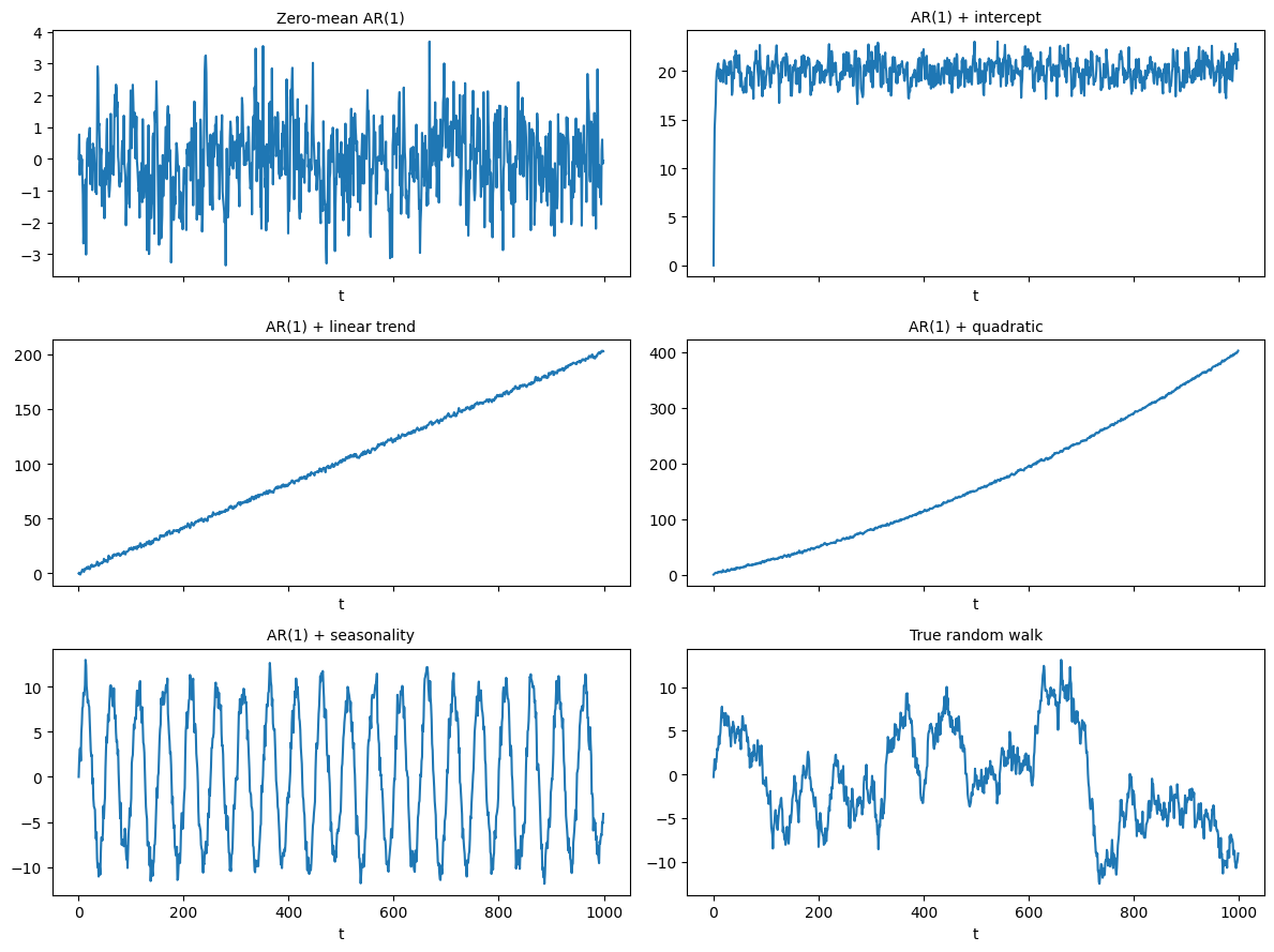
The plots below visualises one realisation of each series at T=1_000.
Dickey-Fuller p-values across four regressions
For each series let's run adfuller(x, maxlag=0, regression=reg) with reg one of {'n','c','ct','ctt'}. We print p-values only, then a four-letter flag: Y if H₀ (unit root) is rejected at 5%, n otherwise. We use T=1_000_000 to avoid spurious results.
The code is below:
# Setup
T = 1_000_000
np.random.seed(654321)
series_funcs = {
    'zero-mean AR(1)': series_n,
    'AR(1) + intercept': series_c,
    'AR(1) + linear trend': series_ct,
    'AR(1) + quad trend': series_ctt,
    'AR(1) + seasonality': series_seasonal,
    'True random walk': random_walk,
}
regressions = ['n', 'c', 'ct', 'ctt']

# Run tests
results = []
for name, func in series_funcs.items():
    x = func(T)
    row = {'Series': name}
    for reg in regressions:
        stat, pvalue, usedlag, nobs, crit = adfuller(x, maxlag=0, regression=reg, autolag=None)
        row[f'{reg}_stat'] = stat
        row[f'{reg}_pvalue'] = pvalue
    results.append(row)

df_results = pd.DataFrame(results).set_index('Series')

# Settings
cols = ['n', 'c', 'ct', 'ctt']
alpha = 0.05

# Build header
header = f"{'Series':<25s}" + "".join(f"{col:>10s}" for col in cols) + f"{'H0 reject?':>12s}"
separator = "-" * len(header)

print(header)
print(separator)

# Print rows
for series_name, row in df_results.iterrows():
    # Gather p-values and rejection flags
    pvals = [row[f"{col}_pvalue"] for col in cols]
    rejects = ['Y' if p < alpha else 'n' for p in pvals]
    summary = "".join(rejects)  # e.g. 'Ynnn'
    # Format p-values to three decimal places
    line = f"{series_name:<25s}"
    for p in pvals:
        line += f"{p:>10.3f}"
    line += f"{summary:>12s}"
    print(line)
Prints:
Series                            n         c        ct       ctt  H0 reject?
-----------------------------------------------------------------------------
zero-mean AR(1)               0.000     0.000     0.000     0.000        YYYY
AR(1) + intercept             0.000     0.000     0.000     0.000        YYYY
AR(1) + linear trend          1.000     0.958     0.000     0.000        nnYY
AR(1) + quad trend            1.000     1.000     0.994     0.000        nnnY
AR(1) + seasonality           0.000     0.000     0.000     0.000        YYYY
True random walk              0.648     0.245     0.080     0.203        nnnn
How to interpret this:
- Zero-mean AR(1): rejects everywhere — no deterministic drift to foul the test.
- Intercept: even the under-specified
'n'regression retains enough power ($\varphi$ well below 1) → alsoYYYY. - Linear trend: succeed once the trend is admitted (
nnYY). - Quadratic drift: needs the full
'ctt'; lesser specs are misleading (nnnY). - Seasonality: a sine wave is not a polynomial, none of the default regressions fit it (
YYYY). - True random walk: happily non-stationary under every specification (
nnnn).
Why is the intercept case YYYY and not nYYY? The intercept itself doesn’t hide the unit-root test the way a time-trend does, so once we give the ADF a huge sample (T = 1_000_000) it still has overwhelming power to reject. The data-generating process:
$ y_t \;=\; \mu \;+\; \varphi\,y_{t-1} \;+\; \varepsilon_t , \qquad \varphi=0.5,\; \varepsilon_t\stackrel{\text{i.i.d.}}{\sim}(0,1) $
Take first differences:
$ \Delta y_t \;=\; \mu \;+\;(\varphi-1)\,y_{t-1}\;+\;\varepsilon_t $
In the ADF regression with regression='n' we estimate
$ \Delta y_t = \gamma\,y_{t-1} + u_t $
The OLS slope is
$ \hat\gamma = \frac{\operatorname{Cov}(y_{t-1},\;\Delta y_t)} {\operatorname{Var}(y_{t-1})} $
Because a constant has zero covariance with $y_{t-1}$, the $\mu$ that appears vanishes from the numerator.
Hence
$ \hat\gamma \xrightarrow{p} (\varphi-1)= -0.5 $
regardless of how large $\mu$ is. So the test statistic remains a large negative number, right in the left tail of the Dickey-Fuller distribution. The way to get this case to be nYYY would be to use a smaller T, to make the standard error larger.
Conclusion
These six toy examples show how easily deterministic quirks — an intercept, a linear or quadratic drift, or a sine-wave seasonality — can fool a unit-root test when the wrong deterministic terms are omitted or over-fitted. Matching the regression option to the data's underlying systemic patterns is therefore important to get right.