Reducing variance in conversion A/B testing with CUPED
Marton Trencseni - Sat 07 August 2021 - ab-testing
Introduction
In the previous post, Reducing variance in A/B testing with CUPED, I ran Monte Carlo simulations to demonstrate CUPED, a variance reduction technique in A/B testing on continuous data, like $ spend per customer. Here I will repeat the same Monte Carlo simulations, but with binary 0/1 conversion data.
The experiment setup is almost entirely the same as in the last post. The only difference is in the get_AB_samples() and get_AB_samples_nocorr() functions, since these now have to generate 0/1 conversion data. The jupyter notebook for this post is up on Github.
Generating correlated conversion data
The approach is to assume a base conversion before_p, say 10%. For each user, do a random 0/1 draw with this probability. This "before" outcome is either 0 or 1. Then, generate the "after" data:
- if the "before" outcome was 0, do a random 0/1 draw with conversion
0 + offset_p, say 10%. This way, most 0s remain 0s. - if the "before" outcome was 1, do a random 0/1 draw with conversion
1 - offset_p, say 90%. This way, most 1s remain 1s. - in the B variant, add
treatment_lift(say 1%) to the above probabilities.
This is just one possible scheme, but it results in "before" and "after" data being correlated. In code:
def draw(p):
    if random() < p:
        return 1
    else:
        return 0

def lmd(x):
    return list(map(draw, x))

def get_AB_samples(before_p, offset_p, treatment_lift, N):
    A_before = [int(random() < before_p) for _ in range(N)]
    B_before = [int(random() < before_p) for _ in range(N)]
    A_after  = [int(random() < abs(x - offset_p))                  for x in A_before]
    B_after  = [int(random() < abs(x - offset_p) + treatment_lift) for x in B_before]
    return lmd(A_before), lmd(B_before), lmd(A_after), lmd(B_after)
We can validate by computing conditional probabilities:
counts = defaultdict(int)
for b, a in zip(A_before, A_after):
    counts[(b, a)] += 1
    counts[(b)] += 1

print('(after = 1 | before = 0) = %.2f' % (counts[(0, 1)]/counts[(0)]))
print('(after = 0 | before = 0) = %.2f' % (counts[(0, 0)]/counts[(0)]))
print('(after = 1 | before = 1) = %.2f' % (counts[(1, 1)]/counts[(1)]))
print('(after = 0 | before = 1) = %.2f' % (counts[(1, 0)]/counts[(1)]))
Prints:
(after = 1 | before = 0) = 0.10
(after = 0 | before = 0) = 0.90 # if it was 0, it's likely to be 0 again
(after = 1 | before = 1) = 0.90 # if it was 1, it's likely to be 1 again
(after = 0 | before = 1) = 0.10
Simulating one experiment
The driver code is, apart from parametrization, the same as before:
N = 10*1000
before_p = 0.1
offset_p = 0.1
treatment_lift = 0.01

A_before, B_before, A_after, B_after = get_AB_samples(before_p, offset_p, treatment_lift, N)
A_after_adjusted, B_after_adjusted = get_cuped_adjusted(A_before, B_before, A_after, B_after)

print('A mean before = %.3f, A mean after = %.3f, A mean after adjusted = %.3f' % (mean(A_before), mean(A_after), mean(A_after_adjusted)))
print('B mean be|fore = %.3f, B mean after = %.3f, B mean after adjusted = %.3f' % (mean(B_before), mean(B_after), mean(B_after_adjusted)))
print('Traditional    A/B test evaluation, lift = %.3f, p-value = %.3f' % (lift(A_after, B_after), p_value(A_after, B_after)))
print('CUPED adjusted A/B test evaluation, lift = %.3f, p-value = %.3f' % (lift(A_after_adjusted, B_after_adjusted), p_value(A_after_adjusted, B_after_adjusted)))
Prints (not deterministic):
A mean before = 0.097, A mean after = 0.179, A mean after adjusted = 0.180
B mean be|fore = 0.099, B mean after = 0.191, B mean after adjusted = 0.190
Traditional    A/B test evaluation, lift = 0.012, p-value = 0.028
CUPED adjusted A/B test evaluation, lift = 0.010, p-value = 0.021
In this particular run, CUPED did a better job approximating the lift with a lower p-value. However, as we saw before, this is not always the case. Although on average CUPED is a better estimator with lower variance, there are experiment runs where CUPED makes the lift measurement worse. For example, after a few re-runs:
A mean before = 0.098, A mean after = 0.178, A mean after adjusted = 0.180
B mean be|fore = 0.103, B mean after = 0.189, B mean after adjusted = 0.187
Traditional    A/B test evaluation, lift = 0.011, p-value = 0.053
CUPED adjusted A/B test evaluation, lift = 0.006, p-value = 0.133
Next, it's interesting to print out the CUPED-transformed variables:
print('Possible mappings:')
mappings = set(['(before=%d, after=%d) -> adjusted=%.3f' % (b, a, p) for
  b, a, p in zip(A_before+B_before, A_after+B_after, A_after_adjusted+B_after_adjusted)])
for m in mappings:
    print(m)
Prints:
Possible mappings:
(before=1, after=0) -> adjusted=-0.722
(before=0, after=1) -> adjusted=1.081
(before=0, after=0) -> adjusted=0.081
(before=1, after=1) -> adjusted=0.278
Remember the CUPED transformation equation was $ Y'_i := Y_i - (X_i - \mu_X) \frac{cov(X, Y)}{var(X)} $. In this equation $\mu_X$, $cov(X, Y)$, and $var(X)$ are constants computed from the experiment results. Both $X_i$ and $Y_i$ can take on two values, 0 or 1, so there are 4 possible combinations, hence $Y'_i$ can take on 4 values. In the above run, the values were -0.722, 1.081, 0.081 and 0.278. It's a bit counter-intuitive, since now the conversion experiment has these weird, even negative values, instead of just 0 and 1.
Simulating many experiments
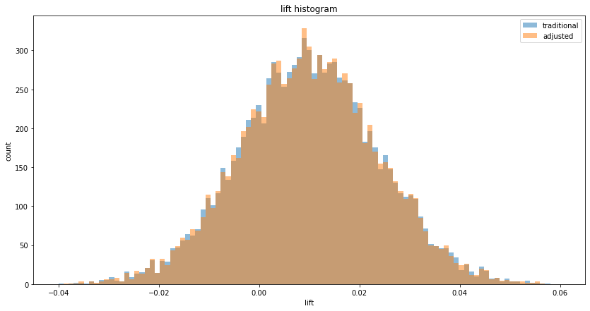
As with continuous variables, CUPED measures the same lift [in conversion], but with lower variance:
Simulating 10,000 A/B tests, true treatment lift is 0.010...
Traditional    A/B testing, mean lift = 0.010, variance of lift = 0.00030
CUPED adjusted A/B testing, mean lift = 0.010, variance of lift = 0.00019
CUPED lift variance / tradititional lift variance = 0.626 (expected = 0.668)
We can observe the tighter lifts on a histogram:
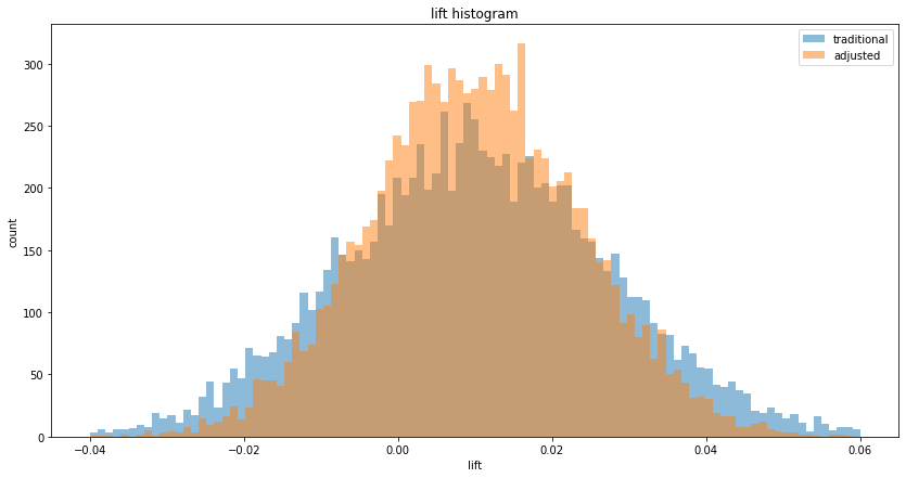
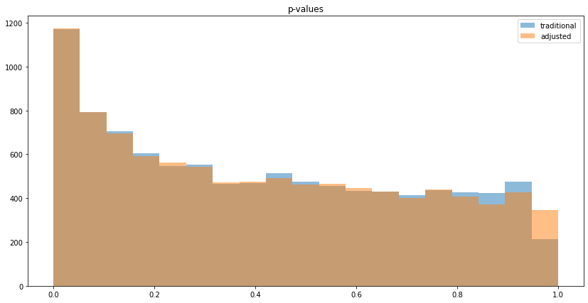
As with continuous variables, the p-values decrease:
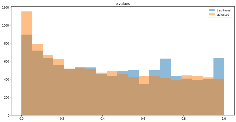
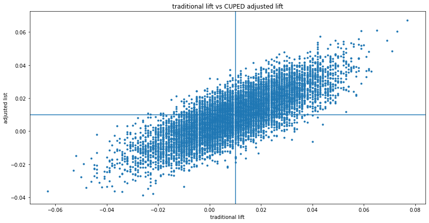
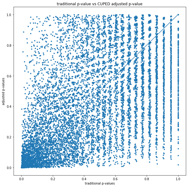
As illustrated above, CUPED lifts and p-values are a better estimate with respect to variance, but not in all cases:
No correlation
The simplest way to generate uncorrelated conversion data is to use random draws independently. In code:
def get_AB_samples_nocorr(before_p, treatment_lift, N):
    A_before = [before_p] * N
    B_before = [before_p] * N
    A_after = [before_p] * N
    B_after = [before_p + treatment_lift] * N
    return lmd(A_before), lmd(B_before), lmd(A_after), lmd(B_after)
Checking conditional probabilities:
P(after = 1 | before = 0) = 0.10
P(after = 0 | before = 0) = 0.90
P(after = 1 | before = 1) = 0.10
P(after = 0 | before = 1) = 0.90
It's uncorrelated, because P(after = 1) = 0.10 in both 0 and 1 before cases, so "after" is independent of "before" (and same for P(after = 0)).
With this generator function, running num_experiments=10,000, we can observe no variance reduction (since "before" and "after" is uncorrelated) on the lift and p-value histograms:
Conclusion
CUPED works for both continuous and binary experimentation outcomes, and reduces variance if "before" and "after" are correlated.