The reward for long-term resilience in simple trading strategies - Part I

Introduction

In this post, I explore how longer-term, more resilient approaches to trading can yield superior returns when using simple, rule-based strategies. Building on my previous discussion on position length, take-profit, and stop-loss dynamics, I compare strategies ranging from daily trades to year-long holds across Nasdaq-100 stocks. By examining metrics like win ratio, mean return, and Sharpe ratio, the data reveals that strategic patience and a willingness to withstand temporary losses can lead to more consistent, risk-adjusted performance over time. The code for this article is available on Github.

Simple trading strategies

In my previous article Stock returns of simple trading strategies, I introduced basic strategies employing position length, take-profit, and stop-loss levels. For example, with symmetric 20% thresholds, if you buy a security at \$100, you would sell when its price reaches either \$120 (take-profit) or \$80 (stop-loss). The take-profit is set because you believe the security isn’t worth more than that price — essentially asking, "Would I buy this security for \$120?" — while the stop-loss protects your funds from larger losses. The position length defines the maximum number of days you’re willing to hold the security before selling at its current market price.

Code

Below is a Python implementation of our trading strategy. The function execute_strategy() iterates over a series of prices and checks whether the take-profit or stop-loss levels have been met. Once either condition is triggered, it returns the exit price and the number of days the position was active. This forms the basis for evaluating both the overall return of the strategy and its normalized daily return.

def execute_strategy(prices, take_profit_price=None, stop_loss_price=None):
    for days, daily_price in enumerate(prices):
        if take_profit_price is not None:
            if daily_price >= take_profit_price:
                return take_profit_price, days+1
        if stop_loss_price is not None:
            if daily_price <= stop_loss_price:
                return stop_loss_price, days+1
    return prices[-1], len(prices)

Once we have the exit information, we compute the return on a trade and normalize it to a mean daily return. Normalization is essential because different strategies might exit at different times, and comparing raw returns would be misleading. For instance, imagine you invest $100 and, over a period of 3 days, that amount grows to $800—an 8x increase. This means the average daily growth factor is 2, because 2 multiplied by itself 3 times (2 × 2 × 2) equals 8. Normalizing returns in this way allows us to compare strategies consistently, even when their holding periods differ.

start_price = ...
final_price, active_days = execute_strategy(...)
r = (final_price - start_price) / start_price
daily_normalized_return = np.exp(np.log(1+r) / active_days) - 1

To simulate a series of trades, the strategy_returns() function applies our trading strategy starting on each day of the price series, returning a list of daily normalized returns. This iterative process helps in understanding the consistency of the strategy over time.

def strategy_returns(prices, position_length, take_profit=None, stop_loss=None):
    returns = []
    for i, start_price in enumerate(prices[:-(position_length)]):
        final_price, active_days = execute_strategy(
            prices=prices[i+1:i+position_length+1],
            take_profit_price=start_price*take_profit if take_profit is not None else None,
            stop_loss_price=start_price*stop_loss if stop_loss is not None else None,
        )
        r = (final_price - start_price) / start_price
        daily_normalized_return = np.exp(np.log(1+r)/active_days)-1
        returns.append(daily_normalized_return)
    return returns

It's straighforward to define a daily_strategy, which simply holds the security for one day, and accepts that day's return:

daily_strategy = lambda prices: strategy_returns(prices, position_length=1, take_profit=None, stop_loss=None)

To analyze investment performance, I compute three statistical measures:

• win ratio: the percentage of days the strategy yields positive returns.
• mean return: the average of the normalized daily returns.
• Sharpe ratio: the mean daily return divided by its standard deviation, indicating risk-adjusted performance.

The corresponding Python code:

def win_ratio(returns):
    return sum(1 for r in returns if r > 0) / len(returns)

def mean_return(returns):
    return np.mean(returns)

def sharpe_ratio(returns):
    return np.mean(returns) / np.std(returns)

Comparing pair of resilient strategies

In this section, I compare two strategies that differ in their resilience—meaning their willingness to hold positions longer or to endure larger temporary losses in pursuit of greater gains. For this analysis, I simulate trades on 100 stocks from the Nasdaq-100 over a 5-year period (2020–2024). The two strategies are:

• daily strategy: buy and sell the next day.
• resilient annual strategy: buy and hold for up to one year (252 trading days) with take-profit and stop-loss set at 50%.

The first is just the daily_strategy as defined above, the second corresponds to strategy_returns(prices, position_length=252, take_profit=1.5, stop_loss=0.5).

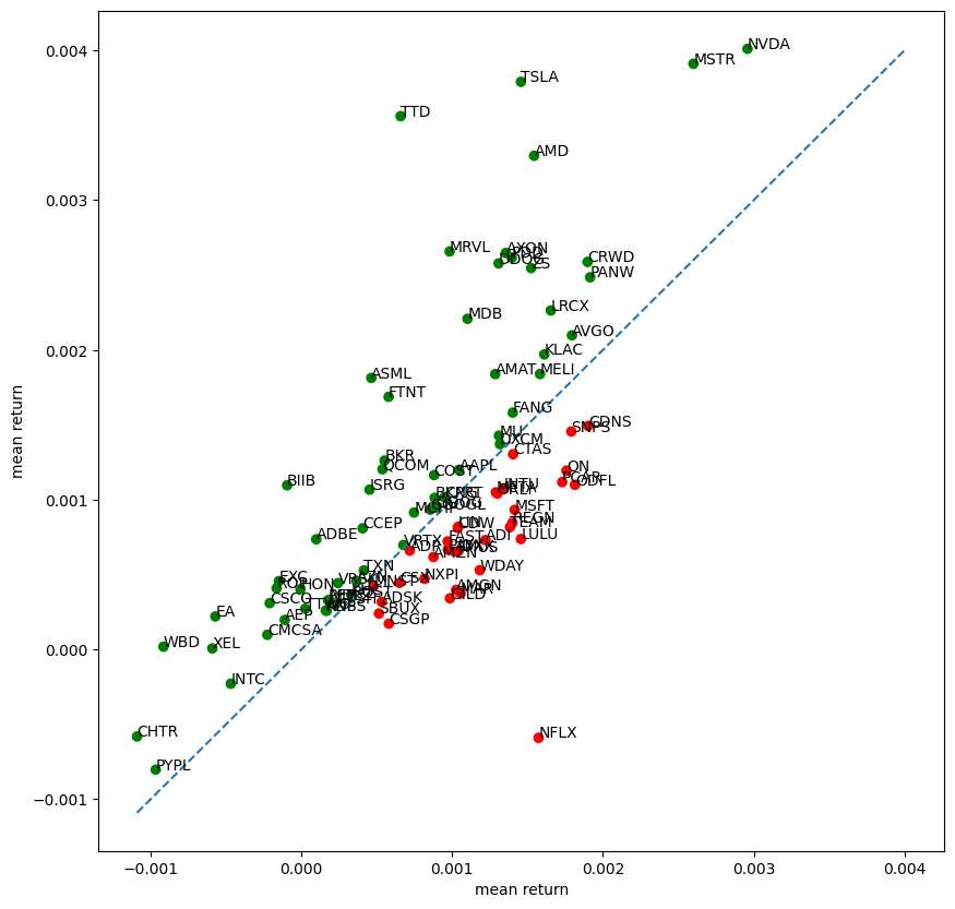
We will start each of the 2 strategies every day for the timeseries of the 100 securities, and record the normalized daily return. In these plots, the more resilient strategy is always on the y-axis, so in this case, the x-axis is for the daily strategy, the y-axis for the resilient annual strategy. Each point (corresponding to a security) is colored green if the resilient strategy yielded a better statistic (above the diagonal), otherwise red. First, let's plot the win ratio (higher is better) of the 2 strategies, for each of the 100 stocks:

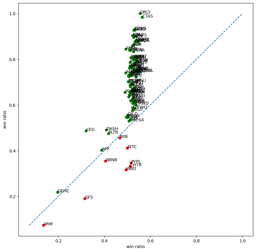
The daily strategy typically achieves about a 50% win ratio, while the resilient approach outperforms it in a higher percentage of cases.

Let's look at the same comparison, but this time use the mean daily return as the statistic on both axis (higher is better):

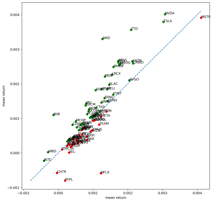
On the mean return chart, it's not clear whether the more resilient strategy is performing better. Next, the Sharpe-ratio (higher is better):

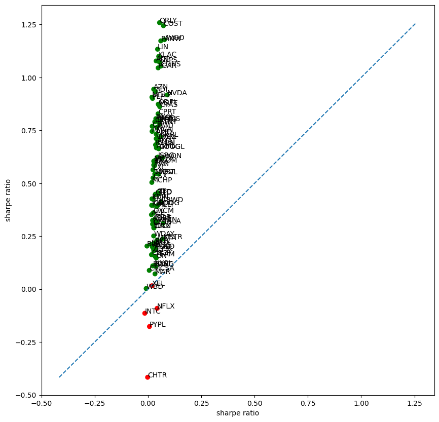
The resilient strategy consistently demonstrates better risk-adjusted returns, with higher Sharpe ratios indicating lower volatility relative to its returns.

Next, I compare two annual strategies with different levels of resilience:

• one using a 10% take-profit and stop-loss (strategy_returns(prices, position_length=252, take_profit=1.1, stop_loss=0.9))
• another using a 50% threshold (strategy_returns(prices, position_length=252, take_profit=1.5, stop_loss=0.5))

The three plots for win ratio, mean daily return and Sharpe ratio are below:

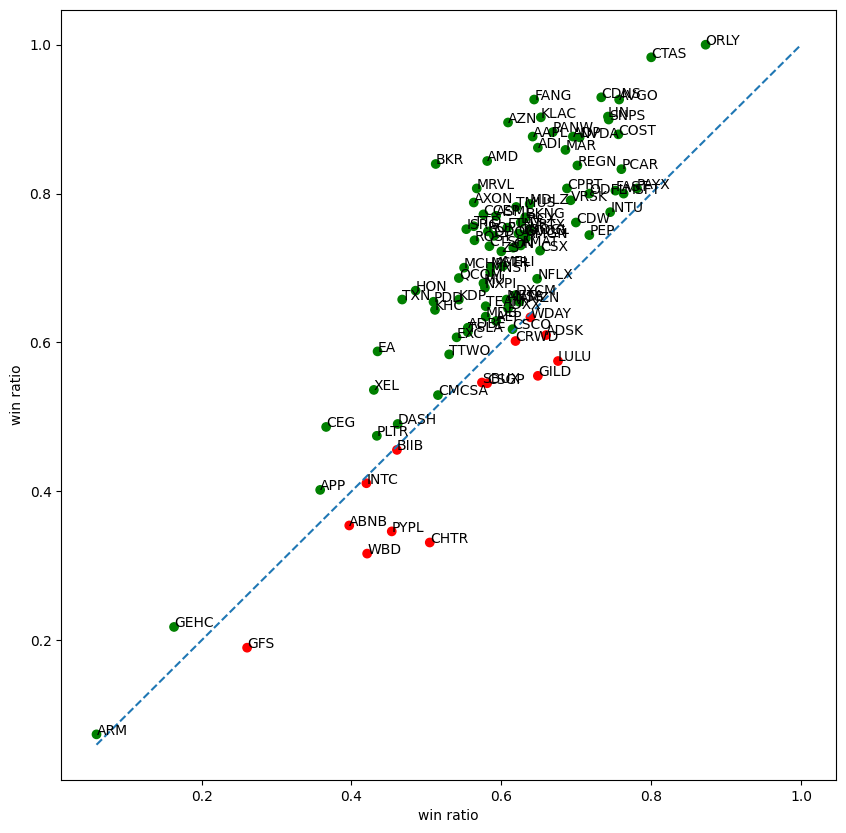
The plots indicate that the more resilient strategy tends to yield better performance across most metrics.

Systematic comparison of strategies

To further understand how resilience influences performance, I systematically compare strategies across different time horizons (1, 3, 6, 9, 12 months). For each horizon, I calculate the difference between the average metric values of the resilient and base strategies (using a 10% take-profit and stop-loss). This “goodness measure” simplifies the comparison across win ratio, mean daily return, and Sharpe ratio.

In other words, we can imagine that we compute the charts above in each case, and subtract the average x value from the average y value (y-x), whether it's win ratio, mean daily return or Sharpe ratio. By reducing each plot to a single goodness measure, we can show multiple strategy comparisons on a single chart. The resulting plots are shown below:

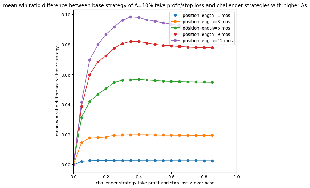
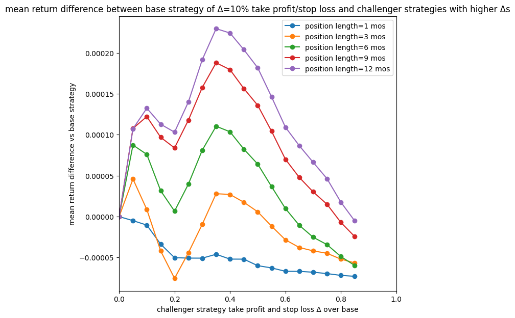
These comparisons yield two key insights:

• Longer horizons tend to capture higher average daily returns compared to shorter ones.
• There is a sweet spot for take-profit and stop-loss thresholds — typically around 40-50% — beyond which performance may begin to decline.

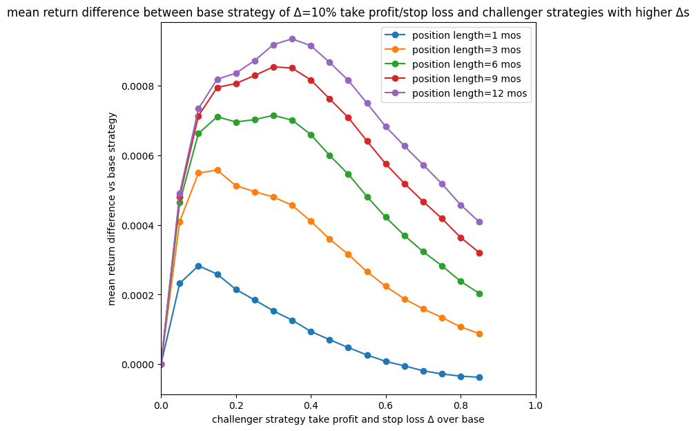
Notably, the mean return plot reveals that setting the take-profit and stop-loss thresholds too high can lead to negative returns compared to the base strategy. This suggests that a less aggressive, asymmetric approach (setting take-profit at a lower percentage than the stop-loss) might offer a better balance between risk and reward. The plot below demonstrates that setting take-profit to half the stop-loss yields smooth, positive mean returns:

Lessons learned

These systematic comparisons reinforce the idea that longer time horizons and greater resilience can enhance performance — not only in raw returns but also in risk-adjusted terms, as indicated by improved Sharpe ratios. However, the relationship is not strictly linear; overly aggressive thresholds can diminish overall returns. This deeper insight emphasizes the importance of fine-tuning strategy parameters to strike the right balance between potential gains and acceptable risk.

Conclusion

These investigations confirm some fundamental principles of investing:

• Longer time horizons generally yield higher returns, win ratios, and Sharpe ratios.
• More resilient strategies — which accept temporary losses in pursuit of larger gains — can deliver superior risk-adjusted performance.
• The optimal ratio between take-profit and stop-loss is rarely 1:1; a more nuanced approach that tolerates greater temporary losses may be necessary to capture significant gains.

Keep in mind that these conclusions are drawn from a specific five-year period in the technology stock market and may not apply under different market conditions.