Stock returns of simple trading strategies
Marton Trencseni - Fri 22 March 2024 - Finance
Introduction
In the previous posts, I looked into the stability of volatilities of various securities, using different volatility measures, and found that there are significant year-over-year differences:
- Introductory investigations into the stability of stock price volatility
- The volatility of simple trading strategy returns
In this article, I clean up the code that I wrote to make it more modular and reusable across experiments.
Tidying the code
First, some helper functions:
def take(series, i):
    return [x[i] for x in series]

def first(series):
    return take(series, 0)

def second(series):
    return take(series, 1)
I don't like working with Pandas DataFrames, I find the API unintuitive --- I prefer working with native Python structures. I'll convert the df returned by yfinance to a list of tuples:
def extract_series(df, ticker, metric):
    return list(zip(list(df.index.astype(str)), list(df_tech[metric][ticker])))
Next, given such a list of stock prices, a helper function to convert it to daily absolute USD returns. This returns a list that is 1 shorter than the input list:
def daily_returns(series):
    return [(series[index][0], (series[index][1] - series[index-1][1]) / series[index-1][1]) for index in range(1, len(series))]
Next, a simple function that converts returns to log-returns. Log-returns are useful, because unlike raw returns, they are additive:
def log_returns(series):
    return [(item[0], log(item[1])) for item in series]
Next, a function that computes returns of a take-profit/stop-loss trading strategy, assuming we have an ensemble of traders, one starting the strategy every day:
def execute_strategy(prices, take_profit_price, stop_loss_price):
    for daily_price in prices:
        if daily_price >= take_profit_price:
            return take_profit_price
        if daily_price <= stop_loss_price:
            return stop_loss_price
    return prices[-1]

def strategy_returns(series, position_length, take_profit, stop_loss, max_price=None):
    returns = []
    prices = second(series) # extract prices
    for i, start_price in enumerate(prices[:-position_length]):
        if max_price is not None and start_price >= max_price:
            continue
        final_price = execute_strategy(
            prices=prices[i+1:i+1+position_length],
            take_profit_price=start_price*take_profit,
            stop_loss_price=start_price*stop_loss
        )
        r = (final_price - start_price) / start_price
        returns.append(r)
    trading_ratio = len(returns)/(len(series)-position_length)
    return list(zip([x[0] for x in series], returns)), trading_ratio
Next, a Python version of GROUP BY, to extract monthly or yearly stats:
def bucketize(series, group_by, compute_func=lambda x:x):
    buckets = defaultdict(lambda: [])
    for (day, r) in series:
        buckets[group_by(day)].append(r)
    return [(key, compute_func(value)) for (key, value) in buckets.items()]
Visualization
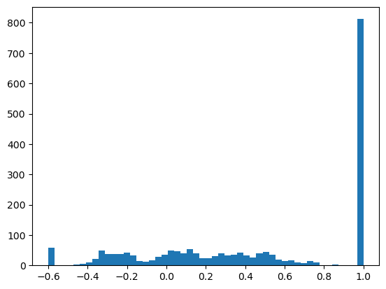
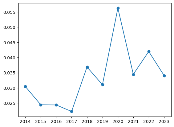
With this, it's simple to reproduce the results from the previous post, but in a modular way:
tickers = ['AAPL', 'MSFT', 'TSLA', 'META', 'GOOG']
df_tech = yf.download(tickers, '2014-01-01', '2023-12-31') # last 10 years

year_days = 262
ticker = 'TSLA'
metric = 'Adj Close'
s = extract_series(df_tech, ticker, metric)
daily_rets = daily_returns(s)
strategy_rets, _ = strategy_returns(s, position_length=2*year_days, take_profit=2, stop_loss=0.4)
daily_rets_per_year = bucketize(daily_rets, group_by=lambda s: s[:4], compute_func=stdev)
pf1 = plt.figure(1)
plt.hist(second(strategy_rets), bins=50)
pf1.show()
pf2 = plt.figure(2)
plt.plot(first(daily_rets_per_year), second(daily_rets_per_year), marker='o')
pf2.show()
Outputs:
Backtesting simple trading strategies
With these helper functions, it's simple to check the historic success of our trading stategies. Let's check them for our favorite 5 tech stocks (['AAPL', 'MSFT', 'TSLA', 'META', 'GOOG']) for the past 5 years. We are willing to hold the position for 1 calendar year, and have a take-profit/stop-loss margin of 50%, what is our win rate (how often do we make a positive return), how often do we enter the position given max_price, what is the average return % (and what is it only counting cases where we actually made a positive return)?
tickers = ['AAPL', 'MSFT', 'TSLA', 'META', 'GOOG']
df_tech = yf.download(tickers, '2019-01-01', '2023-12-31') # last 5 years

position_length=1*year_days
take_profit=1.50
stop_loss=0.5
max_price = None
print(f'PARAMS: take profit={take_profit:.2f}, stop loss={stop_loss:.2f}, position length={position_length}, max price={max_price}')

for ticker in tickers:
    strategy_rets, trading_ratio = strategy_returns(
        extract_series(df_tech, ticker=ticker, metric='Adj Close'),
        position_length=position_length,
        take_profit=take_profit,
        stop_loss=stop_loss,
        max_price=max_price,
    )
    win_rate = mean([int(r > 0) for r in second(strategy_rets)])
    avg_return = mean([r for r in second(strategy_rets)])
    avg_return_cond_win = mean([r for r in second(strategy_rets) if r > 0])
    print(f'ticker={ticker} -> trading ratio={trading_ratio:.2f}, win rate={win_rate:.2f}, avg return={avg_return:.2f}, when winning={avg_return_cond_win:.2f}')
Prints:
PARAMS: take profit=1.50, stop loss=0.50, position length=262, max price=None
ticker=AAPL -> trading ratio=1.00, win rate=0.88, avg return=0.30, when winning=0.35
ticker=MSFT -> trading ratio=1.00, win rate=0.81, avg return=0.29, when winning=0.39
ticker=TSLA -> trading ratio=1.00, win rate=0.72, avg return=0.21, when winning=0.48
ticker=META -> trading ratio=1.00, win rate=0.63, avg return=0.08, when winning=0.38
ticker=GOOG -> trading ratio=1.00, win rate=0.73, avg return=0.19, when winning=0.34
So this strategy had a pretty good win rate in the tech sector recently. As a trader, we can be smarter, and only start such a strategy if the price is "low". Let's define "low" as the mean of the price over this 5 year period (note that this logic is leaking the future into the past):
tickers = ['AAPL', 'MSFT', 'TSLA', 'META', 'GOOG']
df_tech = yf.download(tickers, '2019-01-01', '2023-12-31') # last 5 years
position_length=1*year_days
take_profit=1.50
stop_loss=0.5
print(f'PARAMS: take profit={take_profit:.2f}, stop loss={stop_loss:.2f}, position length={position_length}')
for ticker in tickers:
    s = extract_series(df_tech, ticker=ticker, metric='Adj Close')
    max_price = mean(second(s))
    strategy_rets, trading_ratio = strategy_returns(s,
        position_length=position_length,
        take_profit=take_profit,
        stop_loss=stop_loss,
        max_price=max_price,
    )
    win_rate = mean([int(r > 0) for r in second(strategy_rets)])
    avg_return = mean([r for r in second(strategy_rets)])
    avg_return_cond_win = mean([r for r in second(strategy_rets) if r > 0])
    print(f'ticker={ticker}, max price={max_price:.1f} -> trading ratio={trading_ratio:.2f}, win rate={win_rate:.2f}, avg return={avg_return:.2f}, when winning={avg_return_cond_win:.2f}')
Prints:
PARAMS: take profit=1.50, stop loss=0.50, position length=262
ticker=AAPL, max price=121.4 -> trading ratio=0.51, win rate=1.00, avg return=0.47, when winning=0.47
ticker=MSFT, max price=231.3 -> trading ratio=0.57, win rate=1.00, avg return=0.46, when winning=0.46
ticker=TSLA, max price=170.9 -> trading ratio=0.48, win rate=0.96, avg return=0.46, when winning=0.50
ticker=META, max price=235.5 -> trading ratio=0.60, win rate=0.82, avg return=0.25, when winning=0.40
ticker=GOOG, max price=98.7 -> trading ratio=0.56, win rate=0.97, avg return=0.38, when winning=0.39
For most of these tech stocks, this strategy would have yielded very good win rates and returns.
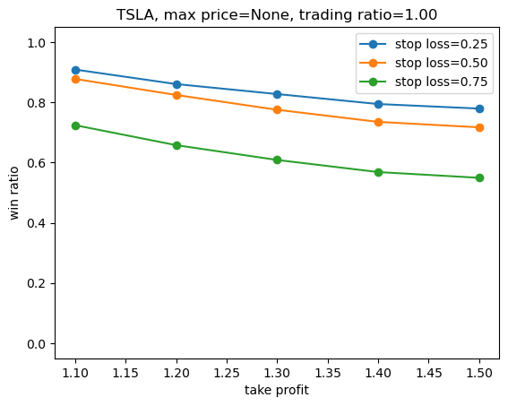
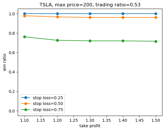
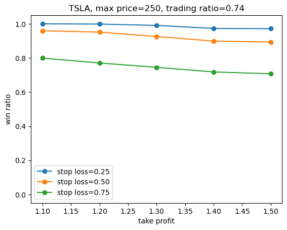
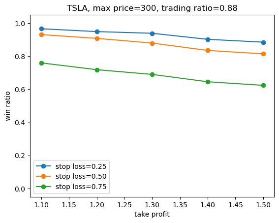
Let's plot the win rate for TSLA as a function of take profit, for different stop loss values. First, a helper function:
def plot_win_rate(df, ticker, metric,
        position_length=1*year_days,
        take_profits = [1.10, 1.20, 1.30, 1.40, 1.50],
        stop_losses = [0.25, 0.50, 0.75],
        max_price=None):
    results = defaultdict(lambda: [])
    s = extract_series(df, ticker, metric)
    for take_profit in take_profits:
        for stop_loss in stop_losses:
            strategy_rets, trading_ratio = strategy_returns(s, position_length, take_profit, stop_loss, max_price)
            win_ratio = mean([int(r > 0) for r in second(strategy_rets)])
            results[stop_loss].append((take_profit, win_ratio))
    # plot:
    legends = []
    for stop_loss, li in results.items():
        legends.append(f'stop loss={stop_loss:.2f}')
        plt.plot(first(li), second(li), marker='o')
    plt.title(f'{ticker}, max price={max_price}, trading ratio={trading_ratio:.2f}')
    plt.xlabel('take profit')
    plt.ylabel('win ratio')
    plt.ylim((-0.05, 1.05))
    plt.legend(legends)
Let's use it:
plot_win_rate(df_tech, ticker='TSLA', metric='Adj Close', max_price=None)
plot_win_rate(df_tech, ticker='TSLA', metric='Adj Close', max_price=200)
plot_win_rate(df_tech, ticker='TSLA', metric='Adj Close', max_price=250)
plot_win_rate(df_tech, ticker='TSLA', metric='Adj Close', max_price=300)
Result:
Conclusion
In retrospect I'm surprised how useful these 10 functions are. Tidying up this code has paid valuable dividends and given me trading ideas. I will continue this series with further investigations of volatility, CAPM and various simple strategies.