White noise into random walks

Introduction

In the previous article, we looked at how the Dickey-Fuller test classifies six sample time series. The first of the time series was of the form:

        $ y_t = \varphi \, y_{t-1} + \varepsilon_t \qquad \varepsilon_t\stackrel{\text{i.i.d.}}{\sim}(0,\sigma^2). $

Clearly, if $\varphi = 0$, this reduces to $y_t = \varepsilon_t$, the time series is a series of independent normals, pure white noise.

On the other hand, if $\varphi = 1$, $y_t = y_{t-1} + \varepsilon_t$, this is a classic random walk, with the steps following a normal distribution.

But what happens if $0 < \varphi < 1$? In the previous article we said that for $\varphi = \frac{1}{2}$ the time series is stationary, but why? Isn't $\varphi = \frac{1}{2}$ like a „half a random walk”?

The code for this article is on Github.

Explanation

The short answer is „no, the $\varphi = \frac{1}{2}$ case is not like half a random walk”. For all $\varphi < 1$, the time series is stationary and oscillates around zero, only at $\varphi = 1$ does it become a random walk. To see why, expand the series:

        $ y_t \;=\; \varepsilon_t \;+\; \varphi\,\varepsilon_{t-1} \;+\; \varphi^{2}\,\varepsilon_{t-2} \;+\; \varphi^{3}\,\varepsilon_{t-3} \;+\; \dots \;=\; \sum_{k=0}^{\infty} \varphi^{k}\,\varepsilon_{t-k}. $

This infinite sum converges if and only if $\left| \varphi \right| < 1$, because the geometric weights $\varphi^k$ then shrink exponentially. To see that the expectation value (mean) of this is zero (when $\left| \varphi \right| < 1$), remember that the expectation value is a linear operation, ie. $\mathbb{E}[X+Y]=\mathbb{E}[X]+\mathbb{E}[Y]$, so the expectation value can be moved into the sum, and that the expectation value of the normals is zero:

        $ \mathbb{E}[y_t] \;=\; \sum_{k=0}^{\infty} \varphi^{\,k}\,\mathbb{E}[\varepsilon_{t-k}] \;=\; \sum_{k=0}^{\infty} \varphi^{\,k}\,\underbrace{0}_{\text{mean of } \varepsilon} \;=\; 0. $

Code

Let's see the same in code. First, the series:

def series_ar1(T, φ):
    y = np.zeros(T)
    for t in range(1, T):
        y[t] = φ * y[t-1] + np.random.randn()
    return y

Then, let's plot it for different $\varphi$ values, for T=1_000 steps:

T = 1_000
np.random.seed(654321)

phis = list(np.round(np.arange(0.0, 1.0, 0.1), 1)) + [0.99, 1.0]
fig, axes = plt.subplots(3, 4, figsize=(14, 9), sharex=True)
axes = axes.ravel()

for ax, φ in zip(axes, phis):
    y = series_ar1(T, φ)
    ax.plot(y, lw=1)
    ax.set_title(f"φ = {φ}", fontsize=10)
    ax.set_xlabel("t", fontsize=8)
    ax.tick_params(axis='both', labelsize=7)

fig.suptitle(f"AR(1) trajectories as φ approaches 1 for T={T:,} timesteps", fontsize=14)
plt.tight_layout(rect=[0, 0.03, 1, 0.95])

This will show something like:

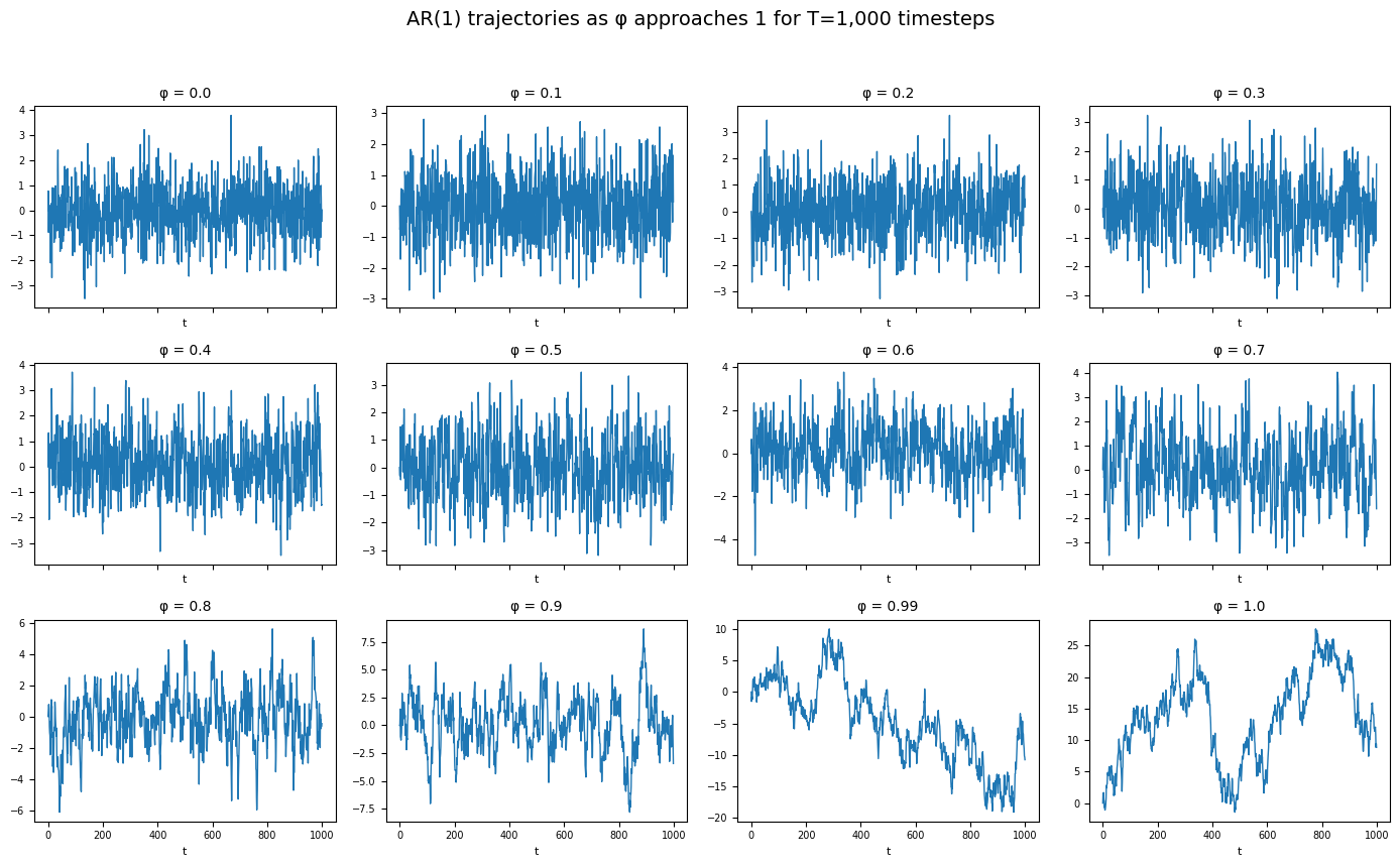
Clearly, for low $\varphi$ values the series oscillates around zero. But for the $\varphi=0.99$ case, it's not so clear. Let's repeat, but with T=1_000_000.

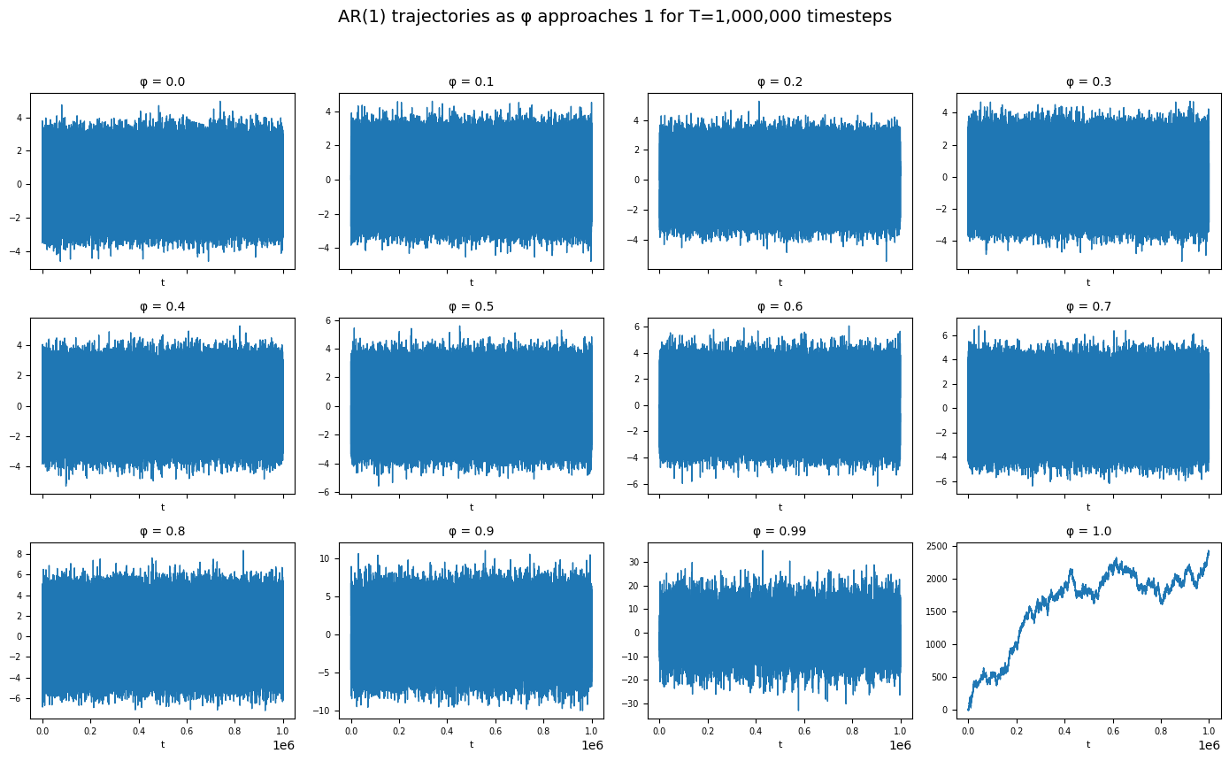
This clearly shows that all series except for $\varphi = 1$ oscillate around zero!

Let's repeat the same, but with $\varepsilon_t \in {+1,-1},\;\; \Pr(\varepsilon_t=1)=\Pr(\varepsilon_t=-1)=\tfrac12$.

def series_ar1(T, φ):
    y = np.zeros(T)
    for t in range(1, T):
        y[t] = φ * y[t-1] + (1 if np.random.random() < 0.5 else -1)
    return y

Plotting again with T=1_000_000:

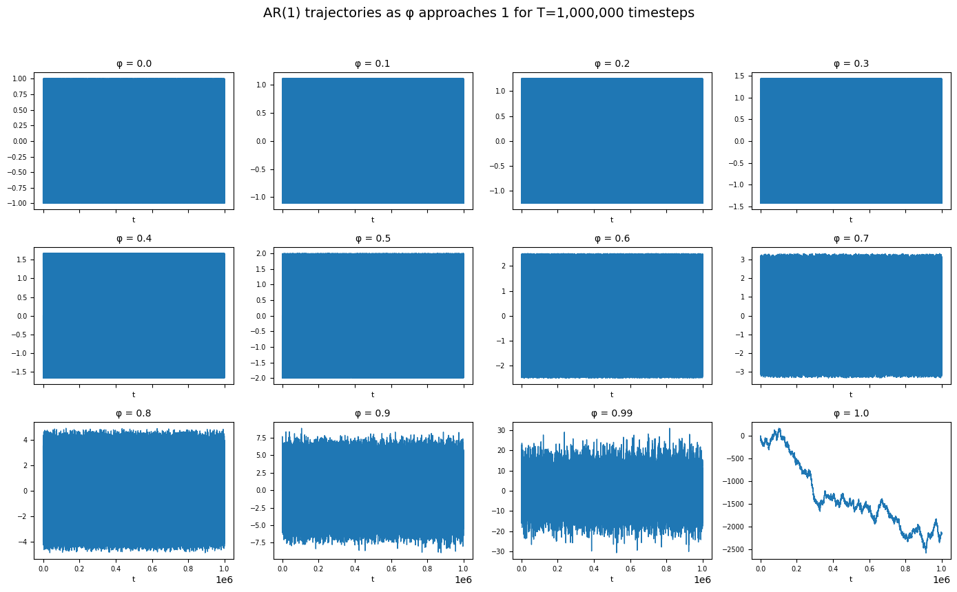
The behaviour in terms of stationarity is the same as for the gaussian case. All variants where $\varepsilon$ has zero mean and finite variance will show this behaviour.

Conclusion

Even when $\varphi = 0.99$, exponential decay of past shocks keeps the variance bounded and the path tethered to its zero mean; random‑walk behaviour only emerges exactly at $\varphi = 1$. Understanding this distinction is essential before applying unit‑root tests to real data, lest slow‑mean‑reverting noise be mistaken for genuine non‑stationarity.