A/A testing and false positives with CUPED

Introduction

In the previous posts, Reducing variance in A/B testing with CUPED and Reducing variance in conversion A/B testing with CUPED, I ran Monte Carlo simulation to get a feel for how CUPED works in continuous (like $ spend per customer) and then binary (conversion) experiments. In both cases, as long as historic "before" and the experiment's "after" data is correlated, CUPED yields lower variance measurements when compared to traditional A/B testing, where only "after" data is used. One of the interesting aspects of CUPED is that although CUPED reduces variance on average, there is no such guarantee for each individual experiment outcome. We saw that on a given experiment outcome, it is possible that the statistics computed from the transformed CUPED variables can be worse than evaluating using just the "after" data using traditional A/B testing:

• the lift computed with CUPED can be lower (or higher), irrespective of what the true lift is
• the p-value computed with CUPED can be lower (or higher), irrespective of what the true lift is

In real-life, Data Scientists are often under pressure to achieve positive results. This poses the potential danger of hacking the experiment, when a Data Scientist computes outcomes with both CUPED and traditional A/B testing and reports the more favorable results, ie. the one with higher lifts and lower p-values. Here I will run Monte Carlo simulations to show (to myself and the reader) that such practice results in incorrect lift measurements and incorrect p-value measurements.

TLDR

The TLDR learning of this post is: as a Data Scientist, we have to pick whether we use traditional A/B testing evaluation (using just "after" data) or CUPED before we evaluate the experiment data, preferably before we even run the experiment. The best case is if there is an experimentation platform which makes this choice for us. As demonstrated below, evaluating both and picking and reporting more favorable results is not statistically sound.

The ipython notebook is up on Github.

Correlated A/A tests

First, let's run an A/A test where "before" and "after" is the same; A/A means there is no difference between A and B, ie. the true lift is 0. I will use the same code as in previous posts, setting treatment_lift=0:

N = 1000
before_mean = 100 
before_sigma = 50
eps_sigma = 20
treatment_lift = 0
num_simulations = 1000
...

Prints:

Simulating 1000 A/B tests, true treatment lift is 0...
Traditional    A/B testing, mean lift = 0.00, variance of lift = 6.09
CUPED adjusted A/B testing, mean lift = 0.03, variance of lift = 0.78
CUPED lift variance / tradititional lift variance = 0.13 (expected = 0.14)

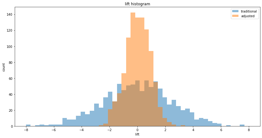
We see that both traditional and CUPED correctly estimate the true lift of 0, but CUPED has lower variance. Plotting the histograms, we see the familiar shape of a narrower CUPED, but this time centered on 0 lift:

Lift hacking

Let's simulate our Data Scientist under pressure in code: at the end of each experiment, we pick and report the higher lift (between traditional and CUPED):

N = 1000
before_mean = 100 
before_sigma = 50
eps_sigma = 20
treatment_lift = 0
num_simulations = 10*1000

print('Simulating %s A/B tests, true treatment lift is %d...' % (num_simulations, treatment_lift))

traditional_lifts, adjusted_lifts, hacked_lifts = [], [], []
for i in range(num_simulations):
    print('%d/%d' % (i, num_simulations), end='\r')
    A_before, B_before, A_after, B_after = get_AB_samples(before_mean, before_sigma, eps_sigma, treatment_lift, N)
    A_after_adjusted, B_after_adjusted = get_cuped_adjusted(A_before, B_before, A_after, B_after)
    traditional_lifts.append(lift(A_after, B_after))
    adjusted_lifts.append(lift(A_after_adjusted, B_after_adjusted))
    hacked_lifts.append(max(
        lift(A_after, B_after),
        lift(A_after_adjusted, B_after_adjusted)
    ))

print('Traditional    A/B testing, mean lift = %.2f, variance of lift = %.2f' % (mean(traditional_lifts), cov(traditional_lifts)))
print('CUPED adjusted A/B testing, mean lift = %.2f, variance of lift = %.2f' % (mean(adjusted_lifts), cov(adjusted_lifts)))
print('Hacked         A/B testing, mean lift = %.2f, variance of lift = %.2f' % (mean(hacked_lifts), cov(hacked_lifts)))

Prints:

Simulating 10000 A/B tests, true treatment lift is 0...
Traditional    A/B testing, mean lift = 0.00, variance of lift = 5.82
CUPED adjusted A/B testing, mean lift = 0.00, variance of lift = 0.80
Hacked         A/B testing, mean lift = 0.89, variance of lift = 2.50

We can see that:

• traditional and CUPED correctly estimate a mean lift of 0
• the hacked result overestimates the lift

We can plot all three on a histogram:

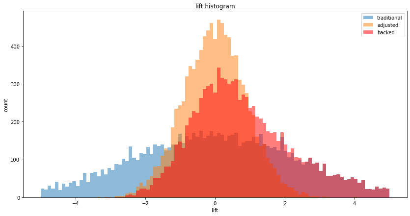
It's a bit hard to see, let's just see the "hacked" histogram:

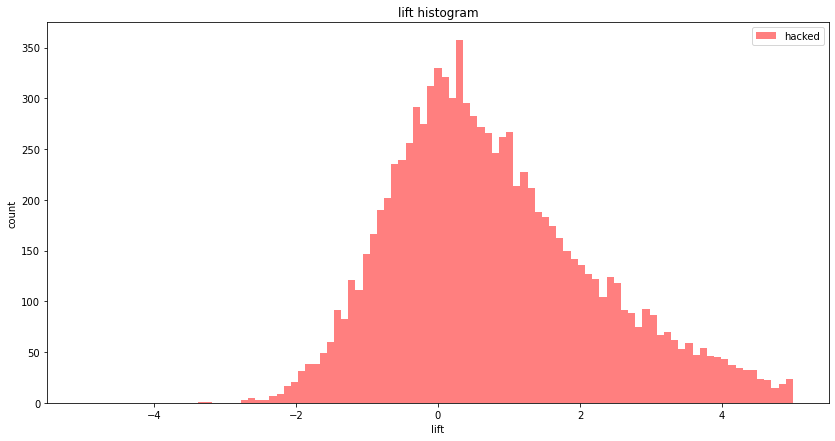
The histogram seems to have its maximum at 0, but it's skewed towards positive values, so on average our imaginary Data Scientist overestimates the lift.

False positive rate

We can now repeat the above logic, and also record the p-value. Our imaginary Data Scientist picks traditional or CUPED adjusted, depending on which has higher lift, and also records that p-value. Let's assume the they use a critical p-value of p_crit = 0.05, so they reject the null hypothesis that A and B are the same, and accept the action hypothesis that B is better. Since A and B are actually the same (since treatment_lift = 0, since we are running A/A tests), these are all false positives.

Let's remember the definition of the p-value. This is the probability of incorrectly rejecting the null hypothesis and accepting the action hypothesis, even though the null hypothesis is true. The null hypothesis is that A and B are the same, ie. an A/A test, which is what we're simulating. So by setting p_crit = 0.05, we are saying we accept a false positive rate (FPR) of 0.05. So if our statistical methodology is sound, repeating our experiment many times (num_simulations), we should get a false positive rate of 0.05. Let's see what happens.

In code:

N = 1000
before_mean = 100 
before_sigma = 50
eps_sigma = 20
treatment_lift = 0
num_simulations = 10*1000
p_crit = 0.05
traditional_fps, cuped_fps, hacked_fps = 0, 0, 0

print('Simulating %s A/B tests, true treatment lift is %d...' % (num_simulations, treatment_lift))

traditional_lifts, adjusted_lifts = [], []
traditional_pvalues, adjusted_pvalues = [], []
for i in range(num_simulations):
    print('%d/%d' % (i, num_simulations), end='\r')
    A_before, B_before, A_after, B_after = get_AB_samples(before_mean, before_sigma, eps_sigma, treatment_lift, N)
    A_after_adjusted, B_after_adjusted = get_cuped_adjusted(A_before, B_before, A_after, B_after)
    adjusted_pvalue = p_value(A_after_adjusted, B_after_adjusted)
    if p_value(A_after, B_after) < p_crit:
        traditional_fps += 1
    if p_value(A_after_adjusted, B_after_adjusted) < p_crit:
        cuped_fps += 1
    if lift(A_after, B_after) < lift(A_after_adjusted, B_after_adjusted):
        if p_value(A_after, B_after) < p_crit:
            hacked_fps += 1
    else:
        if p_value(A_after_adjusted, B_after_adjusted) < p_crit:
            hacked_fps += 1

print('False positive rate (expected: %.3f):' % p_crit)
print('Traditional: %.3f' % (traditional_fps/num_simulations))
print('CUPED:       %.3f' % (cuped_fps/num_simulations))
print('Hacked:      %.3f' % (hacked_fps/num_simulations))

Prints:

Simulating 10000 A/B tests, true treatment lift is 0...
False positive rate (expected: 0.050):
Traditional: 0.049
CUPED:       0.047
Hacked:      0.073

We see that both with traditional and CUPED, we get around the expected 0.05. However, when we hack our experiment evaluation and pick and choose, our FPR is significantly higher. This demonstrates that pick and choose is not statistically sound: we both overestimate the lift and have a higher false positive rate!

No correlation

In the above case, we were running A/A tests on data where the "before" and "after" was correlated. What happens if we do the same when there's no correlation? Recall that the transformation equation for CUPED is:

$ Y'_i = Y_i - (X_i - \mu_X) \frac{cov(X, Y)}{var(X)} $

If there is no correlation, $cov(X, Y) \approx 0$, so $Y'_i \approx Y_i$. I write $\approx$ for approximate equality instead of equality, because even if there is no correlation, numerically $cov(X, Y)$ won't exactly equal 0, it will be some small number, like 0.001. But still, the transformed $Y_i'$ values will be very close to the original $Y_i$ values, so the lifts (traditional vs. CUPED) will also be very close, as will the p-values. So the above pick and choose hacking will not "work" here, since the two choices (lifts) will be very close, almost the same. We can see this if we run many experiments, and for each one we plot both the traditional and CUPED computed lifts. It's a tight fit to the $y=x$ line:

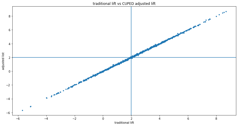
If we repeat the A/A tests above, but with uncorrelated data:

Simulating 10000 A/B tests, true treatment lift is 0...
False positive rate (expected: 0.050):
Traditional: 0.050
CUPED:       0.049
Hacked:      0.050

We see that hacking doesn't work.

Conclusion

The Monte Carlo simulations show explicitly that we have to pick whether we use traditional A/B testing evaluation (using just "after" data) or CUPED before we evaluate the experiment data, preferably before we even run the experiment. As demonstrated in this post, evaluating using both and picking the one with more favorable results is not statistically sound.