A/B testing and the Central Limit Theorem

Introduction

Data Scientists run lots of A/B tests, whether they’re working on SaaS products, social networking, logistics or self-driving cars. A/B testing is a form of hypothesis testing, a decision-making method powered by statistics. By following the rules of hypothesis testing we make sure we have gathered enough and strong enough evidence to support our decisions.

When working with hypothesis testing, the desciptions of the statistical methods often have normality assumptions. For example, the Wikipedia page for the z-test starts like this:

A Z-test is any statistical test for which the distribution of the test statistic under the null hypothesis can be approximated by a normal distribution.

This a common source of confusion. What does it mean that “the test statistic under the null hypothesis can be approximated by a normal distribution”? And whatever that is, how do I know it’s a valid assumption for my data?

The code shown below is up on Github.

A/B testing

Let’s take a concrete example. Suppose we’re doing an A/B test, and we’re measuring two metrics for variants A and B: a $C$ conversion rate (at what rate do people convert) and a $T$ timespent (how many minutes do they spend in the product). In both case, our null hypothesis would be “A and B are the same”, which is translated into the language of mathematics like:

• $ H_0 $ null hypothesis for conversion rate: $ C_A = C_B $
• $ H_0 $ null hypothesis for timespent: $ T_A = T_B $

Here comes the important part: in the above expression, $ C_A $ and $ C_B $ are the conversion rate, and $ T_A $ and $ T_B $ are the average timespent minutes. Both of these quantities are averages: for the conversion rate, we can imagine a conversion counting as a 1 and a non-conversion as a 0, and the conversion rate is the average of this random variable (like coinflips). The timespent is also computed by adding up the individual timespent minutes and dividing by the number of samples.

And this is the key: the z-test works only if these averages can be approximated by a normal distribution. So it’s not the distribution of conversions or the distributions of timespents which must be normal. In fact, these do not follow a normal distribution at all! The conversions are 0s and 1s and follow a Bernoulli distribution, like coin tosses. Timespents usually follow an exponential-looking drop-off in SaaS products. But, given a big enough sample size, the distribution of averages computed from samples can in fact be approximated by a normal. This is the guarantee of the Central Limit Theorem (CLT).

The test statistic is actually the difference of the means: for example, $ T_A = T_B $ can be reformulated as $ T_A - T_B = 0 $, and it is this difference (normalized) that is the test statistic. Fortunately, independent normal distributions have a very nice additive property: if $ X $ and $ Y $ are independent normal random variables, then $ Z_+ = X + Y $ and $ Z_- = X - Y $ are also normals. So if $ T_A $ and $ T_B $ are normal, so is the test statistic $ T_A - T_B $.

The Central Limit Theorem

Without further ado, the Central Limit Theorem:

In probability theory, the central limit theorem (CLT) establishes that, in some situations, when independent random variables are added, their properly normalized sum tends toward a normal distribution (informally a "bell curve") even if the original variables themselves are not normally distributed. The theorem is a key concept in probability theory because it implies that probabilistic and statistical methods that work for normal distributions can be applicable to many problems involving other types of distributions.

For example, suppose that a sample is obtained containing many observations, each observation being randomly generated in a way that does not depend on the values of the other observations, and that the arithmetic mean of the observed values is computed. If this procedure is performed many times, the central limit theorem says that the distribution of the average will be closely approximated by a normal distribution. A simple example of this is that if one flips a coin many times the probability of getting a given number of heads in a series of flips will approach a normal curve, with mean equal to half the total number of flips in each series; in the limit of an infinite number of flips, it will equal a normal curve.

In layman’s terms, the CLT says that: given a population P, with some metric M whose true average is $ \mu_M $, and you take a random sample of independent measurements from P and take the average $ a_M $, then $ a_M $ follows a normal distribution. Note that the error of the measurement, $ e_M = \mu_M - a_M $ also follows a normal distribution since $ \mu_M $ is a constant. $ e_M $ is the quantity most closely related to the $ H_0 $ null hypothesis' test statistic.

Monte Carlo simulation

We can "prove" this to ourselves by running Monte Carlo simulations:

1. First, we will define a population with some distribution. It doesn’t have to be normal, it can be uniform, exponential, whatever.
2. Then we take sample_size samples and compute the mean.
3. We do the above step num_sample times, so we have num_sample means.
4. Then we plot these means and according to the CLT, we should see a nice bell curve centered on the true mean of the original population distribution (ie. the mean of the uniform, the mean of the exponential, etc).

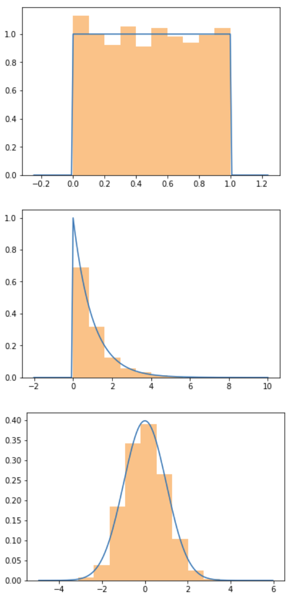
Let's use scipy, it gives us convenient ways to sample standard distributions. First, a function which samples a given distribution and shows a histogram of the samples against the probability density function of the distribution. We can use this to check that we're doing the right thing:

def population_sample_plot(population, sample_size=1000):
    sample = population.rvs(size=sample_size)
    padding = (max(sample) - min(sample)) / 4.0
    resolution = (max(sample) - min(sample)) / 100.0
    z = np.arange(min(sample) - padding, max(sample) + padding, resolution)
    plt.plot(z, population.pdf(z))
    plt.hist(sample, density=True, alpha=0.5)
    plt.show()

Let's visualize a uniform, an exponential and a normal distribution using the above function:

population_sample_plot(uniform)
population_sample_plot(expon)
population_sample_plot(norm)

So these are the original population distributions, and we're trying to estimate the mean by drawing samples. Let's write code to do this:

def population_sample_mean_plot(population, sample_size=1000, num_samples=1000):
    sample_means = [mean(population.rvs(size=sample_size)) for _ in range(num_samples)]
    mn = min(sample_means)
    mx = max(sample_means)
    rng = mx - mn
    padding = rng / 4.0
    resolution = rng / 100.0
    z = np.arange(mn - padding, mx + padding, resolution)
    plt.plot(z, norm(mean(sample_means), std(sample_means)).pdf(z))
    plt.hist(sample_means, density=True, alpha=0.5)
    plt.show()

Let's see the distribution of the means for the same three distributions:

population_sample_mean_plot(uniform)
population_sample_mean_plot(expon)
population_sample_mean_plot(norm)

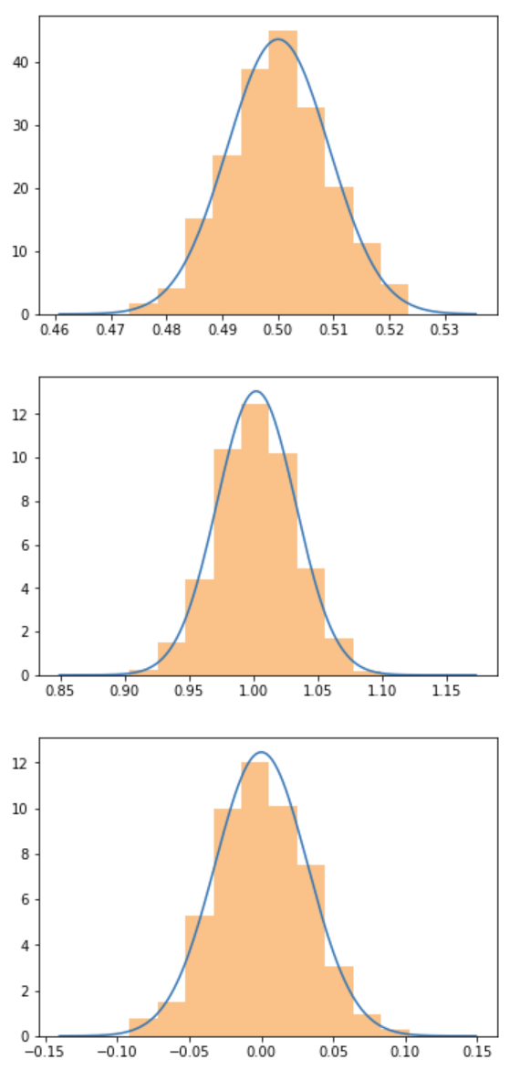
The Central Limit Theorem works!The distribution of the means, for uniform, exponential and normal distributions is a normal distribution, about the true population mean.

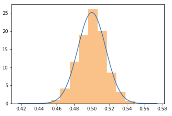
Note that the CLT also works for discrete distributions such as the Bernoulli distribution, the underlying distribution for conversions.

population_sample_mean_plot(bernoulli)

Standard error

The CLT says that the means follow a normal distribution centered around the true mean of the population. What about the width of the bell curve? The technical term for the width of a distribution is the standard deviation. Furthermore, there is a dedicated term for the standard deviation of a sample drawn to estimate a population parameter such as the mean, we call this the standard error:

The standard error (SE) of a statistic (usually an estimate of a parameter) is the standard deviation of its sampling distribution[1] or an estimate of that standard deviation. If the parameter or the statistic is the mean, it is called the standard error of the mean (SEM). The sampling distribution of a population mean is generated by repeated sampling and recording of the means obtained. This forms a distribution of different means, and this distribution has its own mean and variance.

Without going into details, the standard error $ s $ is $ s = \sigma / \sqrt{N} $, where $ \sigma $ is the standard deviation of the original population, and $ N $ is the sample size (sample_size in the code above). Aas we draw more and more samples (more $ N $), the standard error $ s $ decreases, so we get a "needle" bell curve around the true population mean. We can get an arbitrarily accurate estimate of the mean by drawing a lot of samples.

Conclusion

The Central Limit Theorem is the reason why, when you're doing A/B testing on averages (such as conversion or average timespents), the normality assumption for hypothesis testing is usually justified. In the next post I will show cases when the CLT does not apply.