Beyond the Central Limit Theorem

Introduction

In the previous post, A/B testing and the Central Limit Theorem, I talked about the importance of the Central Limit Theorem (CLT) to A/B testing. Here we will explore cases when we cannot rely on the CLT to hold. Exploring when a theorem doesn’t hold is a good way to deepen our understanding why the theorem works when it works. It’s a bit like writing tests for software and trying to break it.

I will show 3 cases when we cannot rely on the CLT to hold:

1. the distribution does not have a mean, eg. the Cauchy distribution
2. violating the independence assumption of the CLT, eg. with a random walk
3. small sample size, eg. when events such as fraudulent transactions have a very low probability

The code shown below is up on Github.

1. The distribution does not have a mean

The CLT says that when we are approximating the mean of a distribution by sampling, the sample means follow a normal distribution. So the CLT is about approximating the mean of a distribution. What if the distribution does not have a mean? In cases like this, we can still sample it, and compute a mean, but:

• since the original distribution doesn't have a mean, we're not approximating it
• the sampled means will not converge to any value, they will keep jumping around

How is it even possible for a distribution not to have a mean? The mean, or expected value $ E[X] $ of a continuous random variable $ X $ with probability density function (pdf) $ f $ is given by:

$ E[X] = \int x f(x) dx $, where $ \int f(x) dx = 1 $

For a discrete random variable:

$ E[X] = \sum i p_i $, where $ \sum p_i = 1 $

The mean of a distribution does not exist if the integral or sum does not exist, ie. for a "pathological" $ f $ or $ p_i $.

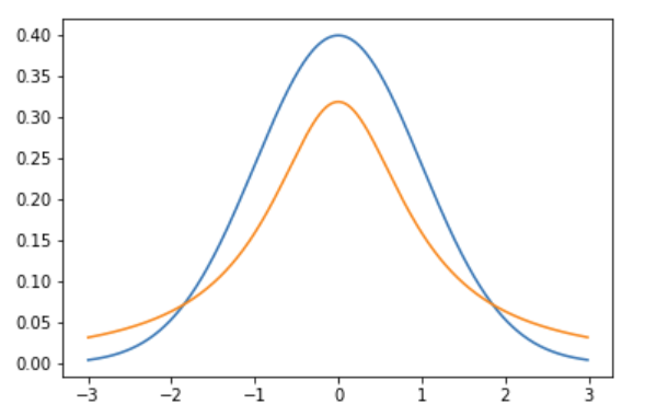
One example is the Cauchy-distribution, defined by $ f(x) = \frac{ 1 }{ \pi ( 1 + x^2 )} $. If you plug this into the above integral, it does not exist.

The Cauchy distribution looks like this (shown with the normal in blue, cauchy in orange; notice how cauchy is more narrow in the center and fatter in the tails than the normal):

We can see this for ourselves with a Monte Carlo simulation:

1. Draw samples from a distribution
2. Every 100 sample, compute the running mean (from the very beginning)
3. Plot the running mean, together with the standard error

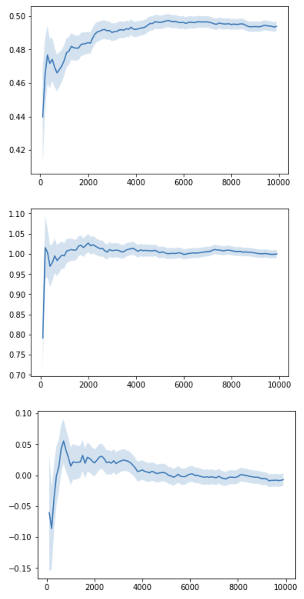
Like in the previous post, we'll use scipy. First let's do this for distributions that have a mean: uniform ($ \mu = 0.5 $), exponential ($ \mu = 1 $) and a standard normal ($ \mu = 0 $):

def population_running_mean_plot(population, sample_size=10*1000):
    sample = population.rvs(size=sample_size)
    step_size = int(len(sample)/100)
    running_stats = []
    for i in range(100, len(sample), step_size):
        running_sample = sample[:i]
        running_stats.append(([i, mean(running_sample), sem(running_sample)]))
    x = [x[0] for x in running_stats]
    y = [x[1] for x in running_stats]
    envelope_min = [x[1] - x[2] for x in running_stats]
    envelope_max = [x[1] + x[2] for x in running_stats]
    plt.plot(x, y)
    plt.fill_between(x, envelope_min, envelope_max, alpha=0.2)
    plt.show()
population_running_mean_plot(uniform)
population_running_mean_plot(expon)
population_running_mean_plot(norm)

Let's see how the running mean converges to the true sample mean after $N=10000$ samples:

Let's do the same for the Cauchy distribution, but let's let it run for $N=10000000$ samples:

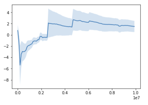
For the Cauchy even after millions of samples, sometimes there is a big jump in the running mean (unlike the previous distributions). It does not converge: if we keep running it, it will keep jumping around, and it will jump to arbitrarily large values.

Why is this? The Cauchy distribution can be visualized like this: imagine drawing the bottom part of a circle (a half-circle) around the center (x=0, y=1). Each time we want to sample a number from the Cauchy distribution, first we pick an angle $ \theta \in ( -\pi/2, \pi/2) $ in a uniform way on the half circle, and then shoot a ray from the center at that $\theta$ angle to the half-circle, and then on to the x-axis. The coordinate of the x-axis intercept is the returned value for the Cauchy sampling. Although the angle $\theta$ is uniform, the ray can shoot arbitrarily far on the x-axis to generate extremely large or small values, and this happens quite often (the fat tail). Note that the normal distribution can also generate arbitrarily small or large values, but at a lower rate, so the mean still exists there.

Another way to see this is to look at a histogram of $N=100000$ draws and compare it with a normal distribution (top is normal, bottom is Cauchy):

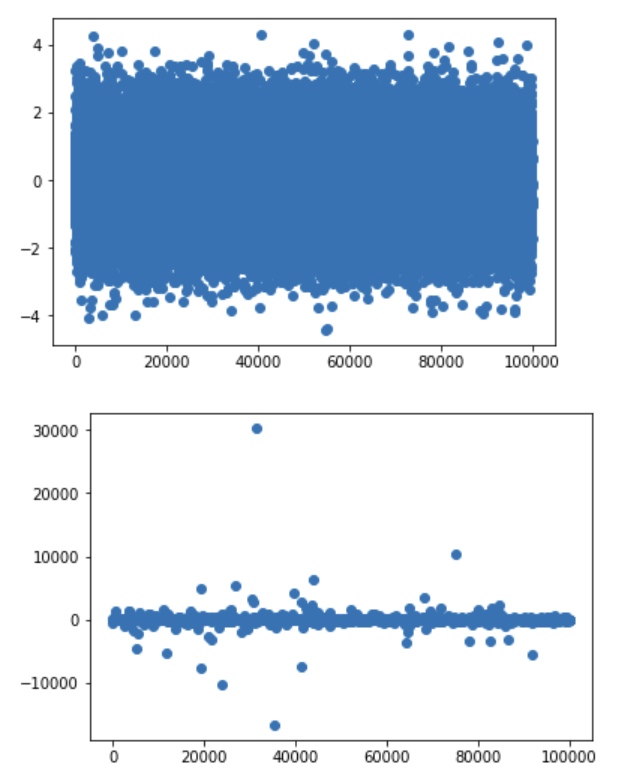
The normal doesn't produce extreme values, whereas the Cauchy does.

2. Violating the independence assumption of the CLT

The wikipedia quote for the CLT starts like this: “...when independent random variables are added...”. In other words, the samples we draw should be independent of each other. What does this mean for an A/B test? For example, if user X and user Y are both using the product, they should not talk to each other, they should not influence each other when making the conversion “decision”, or when "deciding" how much time to spend with the product.

A simple thought experiment that shows how dependence breaks the CLT is the following: suppose a sociology PhD student is taking a salary survey, she sits in a room, test subjects go in and tell her their salary figure (like $50,000), she records it, they leave the room, and the next person goes in. Now suppose that the person who is about to go in asks the person who just left what salary number they said. Then, because they want to look good, they decide to inflate their number and say a bigger number than the previous person, just to impress the sociology PhD student. Putting aside the fact that the survey is flawed, the poor student, if she keeps a running mean of salaries, will see that it keeps going up, and it doesn’t converge. The problem is that she gave her subjects a chance to communicate, and the individual measurements are no longer independent. She needs to have 2 doors, one for incoming and one for outgoing subjects, and make sure people don’t talk to each other.

In statistics, we can construct a similar case by using a random walk: a frog starts at 0, and either goes to +1 or -1 with even probabilities, and so on. We can imagine the frog’s position to be the draws of a distribution, and clearly the subsequent draws are not independent: if the $t=42$ draw was 13 (the frog was at position 13 after 42 time steps), the $t=43$ draw is going to be either 12 or 14, it’s conditioned on the previous draw(s). Similarly to the PhD student’s case, if we keep sampling these numbers and compute the mean, it will not converge. Note that this is not the same as the Cauchy case: here, at each step $t$ (so each random variable in the series) the mean exists and is finite; the mean position at $t=42$ or $t=43$ can be computed and it’s a finite number (it must be 0, see below). But averaging these dependent random variables yields a random variable that breaks the CLT, because the sum does not converge.

Let's see this in action:

def random_walk_draw(num_steps):
    return np.cumsum(2*(bernoulli(p=0.5).rvs(size=num_steps)-0.5))
    #return np.cumsum(norm().rvs(size=num_steps)) # we can also generate the steps with a std. normal

def random_walk_running_mean_plot(sample_size=10*1000, martingale_normalize=False):
    sample = random_walk_draw(num_steps=sample_size)
    step_size = int(len(sample)/100)
    running_stats = []
    for i in range(100, len(sample), step_size):
        running_sample = sample[:i]
        if martingale_normalize:
            m = mean(running_sample)/sqrt(i)
        else:
            m = mean(running_sample)
        running_stats.append(([i, m, sem(running_sample)]))
    x = [x[0] for x in running_stats]
    y = [x[1] for x in running_stats]
    envelope_min = [x[1] - x[2] for x in running_stats]
    envelope_max = [x[1] + x[2] for x in running_stats]
    plt.plot(x, y)
    plt.plot(sample)
    plt.fill_between(x, envelope_min, envelope_max, alpha=0.2)
    plt.show()

random_walk_running_mean_plot(sample_size=10*1000*1000)

Even after $t=10000000$ steps, the running mean is still moving around (orange is the random walk itself, blue is the running mean):

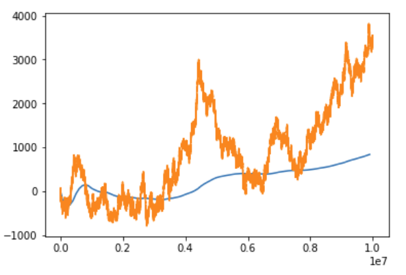
Two interesting notes here:

A. As I mentioned, the mean at any $t$-th timestep in the random walk can be sampled, it exists, and the CLT works. This is because up until the $t$-th timestep, the frog can only get $t$ steps away from the origin ($-t$ or $t$), so at any $t$, the probability distribution is bounded, and the mean exists, and it will be 0 (the true population mean). We can see this for ourselves:

def random_walk_sample_mean_plot(sample_size=1000, num_samples=1000):
    sample_means = [mean(random_walk_draw(num_steps=sample_size)) for _ in range(num_samples)]
    mn = min(sample_means)
    mx = max(sample_means)
    rng = mx - mn
    padding = rng / 4.0
    resolution = rng / 100.0
    z = np.arange(mn - padding, mx + padding, resolution)
    plt.plot(z, norm(mean(sample_means), std(sample_means)).pdf(z))
    plt.hist(sample_means, density=True, alpha=0.5)
    plt.show()

random_walk_sample_mean_plot(sample_size=10*1000, num_samples=1000)

At $t=10000$ steps:

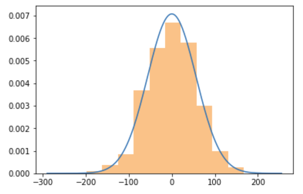
If you're a physicist, you'll know that the standard error is $s=100$, because $s=\sqrt(t)$ for such a random walk, see below.

B. Cases like the random walk can be handled by an extension to the CLT called the Martingale Central Limit Theorem. It essentially says that if you normalize the mean by a suitable function of the steps, then the mean will converge and exists:

In probability theory, the central limit theorem says that, under certain conditions, the sum of many independent identically-distributed random variables, when scaled appropriately, converges in distribution to a standard normal distribution. The martingale central limit theorem generalizes this result for random variables to martingales, which are stochastic processes where the change in the value of the process from time t to time t + 1 has expectation zero, even conditioned on previous outcomes.

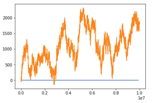
Because simple a random walk, after $ t $ timesteps will on average be $ \sqrt{t} $ steps away from the origin, the normalizing factor is $ \sqrt{t} $. With this, the normalized mean converges to 0. It must be 0 because the whole setup is symmetric around the origin (orange is the random walk itself, blue is the running mean)::

random_walk_running_mean_plot(sample_size=10*1000*1000, martingale_normalize=True)

But note that this is no longer the original CLT. Random walks like this are closely related to Brownian motion, which is what earned Einstein the Nobel price.

3. Small sample size

We also cannot rely on the CLT when the sample size is small. The CLT says that as we increase the sample size $N$, we get arbitrarily close to a normal distribution (even though we never reach it, only in the $ N \rightarrow \infty $ infitinity limit). In real life, we don’t have infinite time, so we always stop at some fixed $N$. It's the Data Scientist's job to make sure we have a big enough $N$ that our approximation is good enough.

Let's use conversions, ie. the Bernoulli distribution as an example, because it illustrates this point in a counter-intuitive, but instructive way. In the previous post we saw that even at $N=1000$ the sample mean nicely approximate a normal... that is, when the $p$ parameter of the Bernoulli is $p=0.5$:

Let's run the same simulation, but at $p=0.001$, with $N=1000$:

population_sample_mean_plot(bernoulli(p=0.001))

We get this:

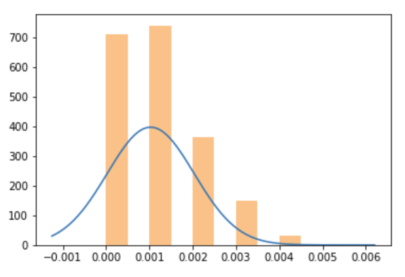
Clearly, this does not (yet) look like a bell curve, and it's strongly asymmetric. What happens is that $Np=1$, so on average we just get 1 conversion. A lot of the time we will get just 0, most often 1, sometimes 2, 3, and so on.. At such low $Np$, we need more samples, so we can more accurately explore the region around the true mean. If we run at say $N=10000$, then $Np=10$, so sometimes we get $0, 1, 2, ... 10 ... $ We get a clearer picture around the average 10.

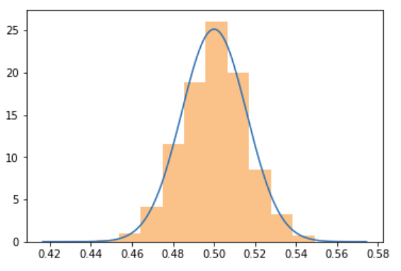
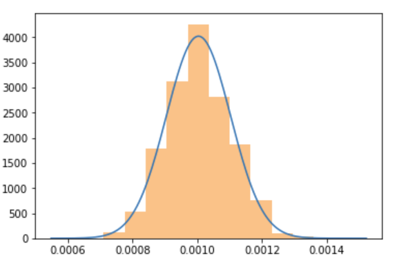
To be clear, the CLT still holds for a low $p$ Bernoulli distribution, we just need to collect more samples, so we get enough conversions per sample to actually see the bell curve. Let's repeat the previous simulation, but at $N=100000$. It shows a beautiful bell curve centered around $p=0.001$:

population_sample_mean_plot(bernoulli(p=0.001), sample_size=100*1000)

So, the CLT still holds, but sometimes we just need to collect more data for it to “start working”. Note that these considerations are baked into sample size calculators such as this.

A good real-life example of working with very low probability events is fraud in credit card transactions. In real life only about 1 in 1,000 transactions are fraudulent. Suppose we're A/B testing an ML model to catch fraudulent transactions: A is the new model, B is the old model. We need to collect a lot of samples to catch enough fraud cases to get a good estimate of the ratios for A and B ($C_A$ and $C_B$ if we think of this as conversions), and the lift between A and B. What the above simulation shows is that if fraud cases happen at $p=0.001$ we will need to collect a lot more samples than if they were to happen at $p=0.5$ frequency.

Conclusion

There are a number of caveats when running A/B tests in real life. Making sure the CLT holds when we use a test statistic that assumes a normal distribution is one of them. From the list of considerations above, the top thing to keep in mind is the concern of sample sizes (#3). In SaaS-like environments, the population distribution will always exist (#1), especially if we winsorize our results (winsorization just means we replace the most extreme values at the two ends of our sample with less extreme values). Independence (#2) usually holds in SaaS environments, but may not in social networks.

It's worth remembering that there are also non-statistical A/B testing errors, eg. if we run variant A in Germany and variant B in France. We may get enough samples for both A and B, both are normals, we get a nice reading on the difference, but we're comparing apples to oranges. We're not measuring (just) the difference between A and B, but the difference between german and french users.