Classification accuracy of quantized Autoencoders with Pytorch and MNIST

Marton Trencseni - Fri 09 April 2021 - Machine Learning

Introduction

In the previous post I investigated the information contents, in bits, that Autoencoders store. I took MNIST digits, trained a simple Autoencoder neural network to first encode the pictures in 4..256 dimensions, where each vector element is a float32. Then I took the elements, and quantized them to 2..32 bits accuracy, and measured the reconstruction loss as a function of encoding dimension and quantization:

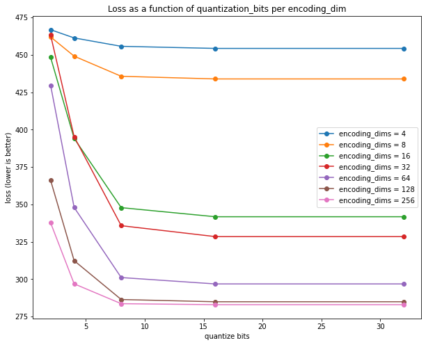
Pytorch Autoencoder loss with encoding dimension and quantization bits

Based on the plot, my conclusion was:

... 512 bits --- which corresponds to 12x (lossy) compression --- is a good trade-off, or 1024 bits for 10% less loss. Loss does not decrease significantly after 1024 bits, that appears to be best the Autoencoder can accomplish.

However, this conclusion is just eye-balled based on the plots leveling off. The y-axis here is loss, which is related to pixel distance between original and reconstruction, but it's actually hard to know what a loss of ~300 really means. Also, this loss is not straightforward pixel distance, since it's standard practice to re-scale and normalize MNIST images to help the neural networks:

tv.datasets.MNIST(..., transform=transforms.Compose([
    transforms.ToTensor(),
    transforms.Normalize((0.1307,), (0.3081,)), <--- image pixels are re-scaled
]))

A better approach to quantify the "loss" is to run a classifier on the output and see how recognizable the digits are in terms of Accuracy %.

The notebook is up on Github.

Experiment setup

The MNIST dataset contains a total of 70,000 digits. Usually the first 60,000 are used for training, the remaining 10,000 for testing. Here, I will use:

30,000 for training a CNN classifier, as in this earlier post
30,000 for training a Autoencoder, like in the previous post
10,000 for testing, how the classifier performs on quantized digits coming from the Autoencoder

Then, I follow the same strategy as previously, but instead of using loss as a metric, I run the quantized Autoencoder's output through the classifier, and plot the accuracy as a as a function of encoding dimension and quantization.

Code

First, some helpers to split the dataset into 3 parts:

class MNISTPartialTrainDataset(Dataset):
    def __init__(self, root, num_samples=None, offset=0):
        self.base_dataset = tv.datasets.MNIST(root=root, train=True, transform=transforms.Compose([
            transforms.ToTensor(),
            transforms.Normalize((0.1307,), (0.3081,)),
        ]))
        if num_samples is None:
            self.num_samples = len(self.base_dataset)
        else:
            self.num_samples = min(num_samples, len(self.base_dataset)-offset)
        self.offset = offset
    def __len__(self):
        return self.num_samples
    def __getitem__(self, idx):
        return self.base_dataset[self.offset+idx]

class MNISTPartialTestDataset(Dataset):
    def __init__(self, root, num_samples=None, offset=0):
        self.base_dataset = tv.datasets.MNIST(root=root, train=False, transform=transforms.Compose([
            transforms.ToTensor(),
            transforms.Normalize((0.1307,), (0.3081,)),
        ]))
        if num_samples is None:
            self.num_samples = len(self.base_dataset)
        else:
            self.num_samples = min(num_samples, len(self.base_dataset)-offset)
        self.offset = offset
    def __len__(self):
        return self.num_samples
    def __getitem__(self, idx):
        return self.base_dataset[self.offset+idx]

The classifier is a vanilla CNN:

class Classifier(nn.Module):
    def __init__(self):
        super(Classifier, self).__init__()
        self.model = nn.Sequential(
            nn.Conv2d(1, 20, 5, 1),
            nn.ReLU(),
            nn.MaxPool2d(2, 2),
            nn.Conv2d(20, 50, 5, 1),
            nn.ReLU(),
            nn.MaxPool2d(2, 2),
            nn.Flatten(),
            nn.Linear(4*4*50, 500),
            nn.ReLU(),
            nn.Linear(500, 10),
            nn.LogSoftmax(),
            )
    def forward(self, x):
        return self.model(x)

We train the classifier on the first 30,000 MNIST digits:

classifier = Classifier().to(device)
distance = nn.NLLLoss()
optimizer = torch.optim.SGD(classifier.parameters(), lr=0.01, momentum=0.5)
num_epochs = 20
for epoch in range(num_epochs):
    for data, target in classifier_dataloader:
        data, target = data.to(device), target.to(device)
        optimizer.zero_grad()
        output = classifier(data)
        loss = distance(output, target)
        loss.backward()
        optimizer.step()
    print('epoch {:d}/{:d}, loss: {:.4f}'.format(epoch+1, num_epochs, loss.item()), end='\r')

correct = 0
classifier = classifier.to('cpu')
for data, target in classifier_dataloader:
    output = classifier(data)
    pred = output.argmax(dim=1, keepdim=True) # get the index of the max log-probability
    correct += pred.eq(target.view_as(pred)).sum().item()
print('Classifier train accuracy: {:.1f}%'.format(100*correct/len(classifier_dataloader.dataset)))

The classifier achieves 99.8% train accuracy, as expected:

Classifier train accuracy: 99.8%

Now the Autoencoder, exactly the same as before:

class Autoencoder(nn.Module):
    def __init__(self, encoding_dims):
        super(Autoencoder,self).__init__()
        self.encoder = nn.Sequential(
            nn.Flatten(),
            nn.Linear(img_dims*img_dims, encoding_dims),
            nn.ReLU(),
            )
        self.decoder = nn.Sequential(
            nn.Linear(encoding_dims, img_dims*img_dims),
            nn.Unflatten(1, (1, img_dims, img_dims)),
            nn.Sigmoid(),
            )
    def forward(self, x, quantize_bits=None):
        x = self.encoder(x)
        x = torch.sigmoid(x)
        if quantize_bits is not None:
            x = round_bits(x, quantize_bits)
        x = torch.logit(x, eps=0.001)
        x = self.decoder(x)
        return x

The main loop is very similar to before, except there is an additional step, where the trained classifier is run on the Autoencoder's output digits:

results = []
for encoding_dims in [4, 8, 16, 32, 64, 128, 256]:
    # train autoencoder, code omitted
    ...
    # test
    for quantize_bits in [None, 2, 4, 8, 16, 32]:
        correct = 0
        autoencoder = autoencoder.to('cpu')
        for imgs, labels in autoencoder_test_dataloader:
            ae_imgs = autoencoder(imgs, quantize_bits=quantize_bits)
            output = classifier(ae_imgs)
            pred = output.argmax(dim=1, keepdim=True) # get the index of the max log-probability
            correct += pred.eq(labels.view_as(pred)).sum().item()
        accuracy = correct/len(autoencoder_test_dataloader.dataset)
        results.append((encoding_dims, quantize_bits, accuracy))

Results

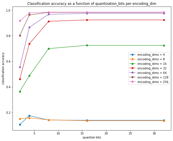
The results can be plotted to show the accuracy of the classifier per encoding_dims, per quantize_bits:

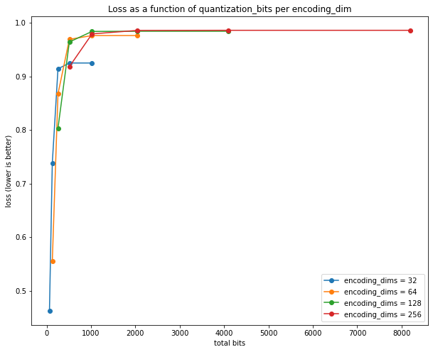
Classifier accuracy on quantized Autoencoder output after quantization

Alternatively we can plot total_bits = encoding_dims * quantize_bits on the x-axis:

Classifier accuracy on quantized Autoencoder output after quantization as a function of total bits

The plots re-affirm what I read off the previous plots, that

each float32 in the encoding stores around 8 bits of useful information (out of 32), since all of the curves flatten out after 8 bits
128 dimensions is the maximum required, since the next jump to 256 yield no significant increase in accuracy
overall, based on these curves, encodim_dims = 64 and quantize_bits = 8 appears to be a good trade-off (total_bits = 64*8 = 512 bits)

However, now it's easier to quantify:

at encodim_dims = 64 and quantize_bits = 8 (total_bits = 64*8 = 512 bits), the classifier achieves 97% accuracy, which is still great
at higher total_bits, and with no quantization at all, the classifier achieves 98% on these unseen, encoded-than-decoded images, which is the same 98% we get without no quantization at all

Finally, to visually see what happens when we autoencode and quantize, a sample of the Autoencoder's output, for encoding_dims=64 and various quantization levels: