Modern Portfolio Theory II: Random portfolio coverage in log volatility—return space with a risk free asset

Introduction

In the previous article Modern Portfolio Theory I: Random portfolio coverage in log volatility—return space, we simulated random portfolios composed of risky assets and explored their distribution in log volatility—return space. This follow-up introduces a risk-free asset into the mix, allowing us to extend the analysis and observe how its inclusion reshapes the overall distribution of portfolio outcomes. By adding this asset, we can now highlight the theoretical link to the Capital Market Line (CML), a core concept in the Capital Asset Pricing Model (CAPM). With a risk-free asset, the efficient frontier transforms into a straight line connecting the risk-free rate and the market portfolio, creating a more structured and predictable environment. This modification not only broadens our understanding of the trade-off between risk and return, but also offers deeper insight into how optimal portfolios adjust when a “safe haven” investment is available. In the sections that follow, I show how incorporating the risk-free asset changes the convex hull of feasible portfolios. The notebook is on Github.

Injecting the risk-free asset into the portfolio

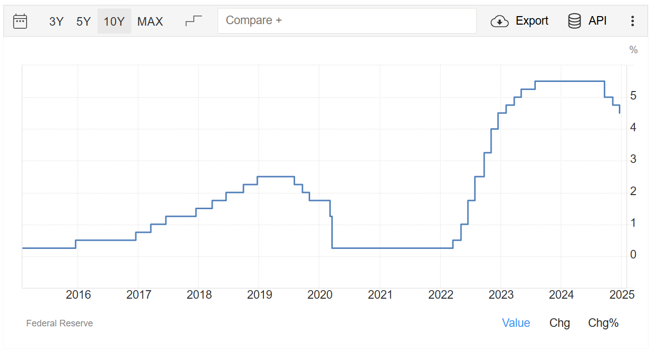
The risk-free asset is commonly represented by short-term U.S. Treasury securities (such as Treasury bills), which are considered free of default risk due to the backing of the U.S. government. The yield on these securities effectively serves as the “risk-free rate” in financial models. In the United States, short-term interest rates are heavily influenced by the Federal Reserve’s monetary policy. The Fed sets a target for the federal funds rate, the overnight lending rate between banks, and uses open market operations—buying and selling existing Treasury securities—to steer that rate toward its target. This action influences a wide range of other interest rates, including the yields on Treasury bills, which in turn shape the baseline risk-free rate used by investors. Historically, short-term interest rates have fluctuated significantly, sometimes reaching into double-digit territory, while in recent years they have remained comparatively low. You can see historic interest rates here. In the last 10 years, the lowest it has been is 0.25%, the highest it has been is 5.5%. For this article, I will assume an annualized 5% interest rate, which corresponds to a daily rate of $R_{daily}=R_{annual}^{1/T}=e^{ln(R_{annual})/T}$, assuming T days of compound interest. In our study, there are 250 trading days, so we have $T=249$ days of return data, so with $R_{annual}=1.05$, numerically $R_{daily}=1.0001959$ and $ln(R_{daily})=0.0001959$.

In terms of the code, we can treat the risk-free asset like any other security, it just happens to have the same daily return every day:

# download 2023 Nasdaq-100 daily closing prices
url = 'https://en.m.wikipedia.org/wiki/Nasdaq-100'
df_nasdaq_100_list = pd.read_html(url, attrs={'id': "constituents"}, index_col='Symbol')[0]
tickers = list(df_nasdaq_100_list.index)
df_nasdaq_100 = yf.download(tickers, '2023-01-01', '2023-12-31')
# 250 trading days
# convert to log returns, reduces days by 1, to 249 trading days
df_logr = np.log(df_nasdaq_100['Adj Close']).diff()[1:]
# add risk-free asset
risk_free_annual_return = 1.05
risk_free_daily_log_return = np.log(risk_free_annual_return**(1/len(df_logr)))
df_logr.insert(len(df_logr.columns), 'RISKFREE', [risk_free_daily_log_return] * len(df_logr))
# regular returns, 249 trading days
df_r = np.exp(df_logr)

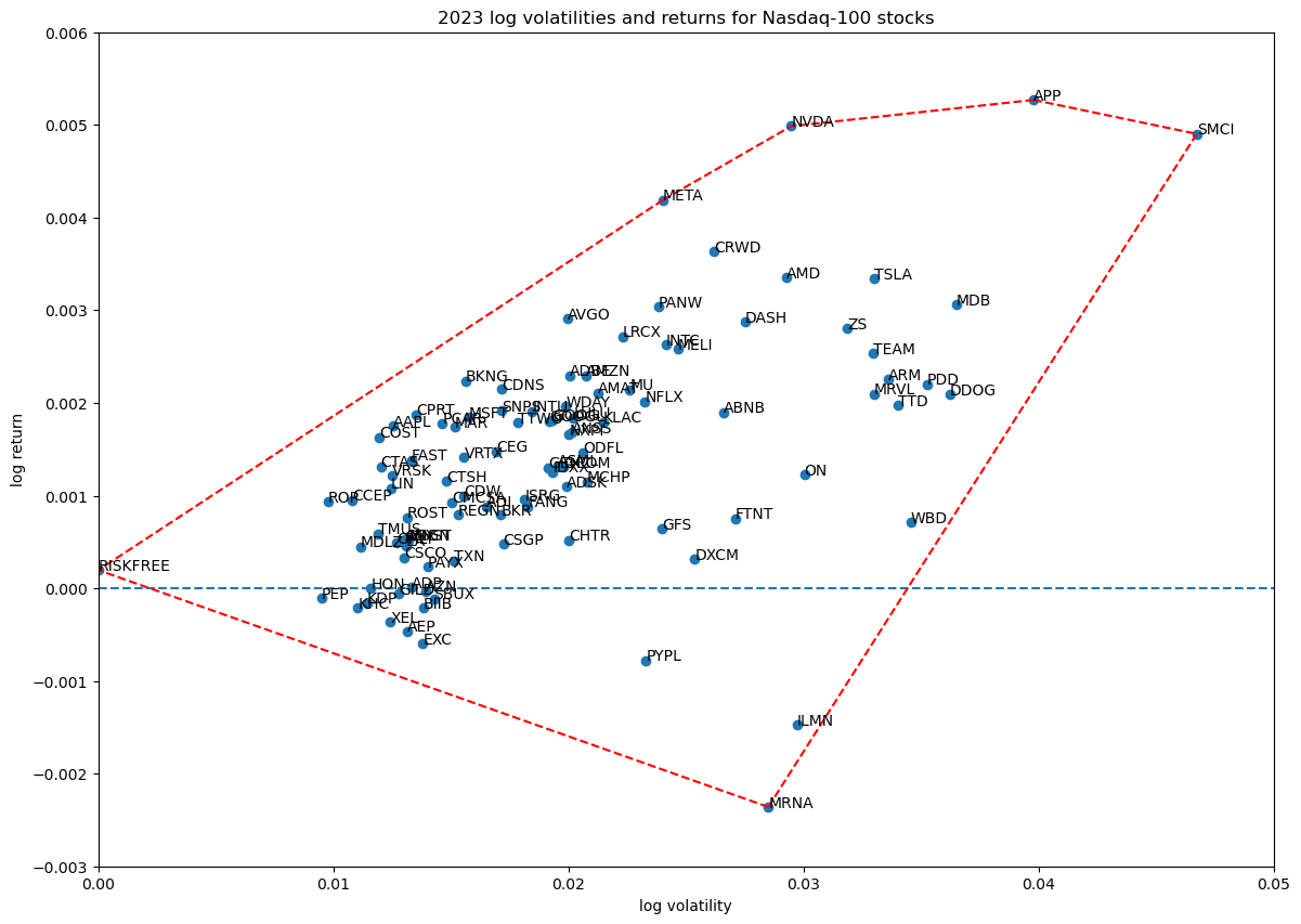
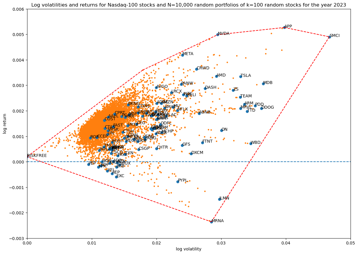
The log volatility—return space of the 100 Nasdaq-100 stocks extended with the risk-free asset is shown below, with their convex hull shown in red:

Randomization strategies

The randomization strategies introduced in the previous article select $k$ random stocks from the overall portfolio space in the Monte Carlo simulation, and distribute weights that sum to unity between these $k$ stocks. One option is to simply use this randomization strategy as-is. The downside is that this treats the risk-free asset as one of $100+1=101$ assets, so we spend a relatively small portion of our Monte Carlo budget on seeing the impact of including the risk-free asset. The alternative is to tweak the portfolio randomization so the risk-free asset is always one of the $k$ selected non-zero weights. In code we achieve this by adding the fix_last parameter (since we appended the RISKFREE column to the end of the dataframe) to random_portfolio():

# make a random portfolio of length num_tickers, with all but portfolio_size tickers zeroed out
def random_portfolio_implementation(num_tickers, portfolio_size=2, fix_last=False):
    if fix_last is False:
        indexes = np.random.choice(np.arange(num_tickers), size=portfolio_size, replace=False)
    else:
        indexes = np.random.choice(np.arange(num_tickers-1), size=portfolio_size-1, replace=False)
        indexes = np.append(indexes, num_tickers-1)
    weight_values = unit_random(portfolio_size)
    portfolio_weights = list(set_weights(num_tickers, indexes, weight_values))
    check_sum = np.sum(portfolio_weights)
    if np.abs(1 - check_sum) > 0.01:
        print(indexes)
        print(weight_values)
        print(portfolio_weights)
        assert(False)
    return portfolio_weights

The original implementation, which does not treat the risk-free asset any differently:

random_portfolio = lambda num_tickers, portfolio_size:
    random_portfolio_implementation(num_tickers, portfolio_size, fix_last=False)

The alternative implementation, which always includes the risk-free asset:

random_portfolio = lambda num_tickers, portfolio_size:
    random_portfolio_implementation(num_tickers, portfolio_size, fix_last=True)

Running the original implementation with $k=5$:

random_portfolio = lambda num_tickers, portfolio_size:
    random_portfolio_implementation(num_tickers, portfolio_size, fix_last=False)
unit_random = unit_random_angle_projection
num_simulations = 10_000
portfolio_size = 5
title = f'...'
portfolios = simulate_portfolios(df_r, portfolio_size, num_simulations)
_ = plot_portfolios(bare, portfolios, title)

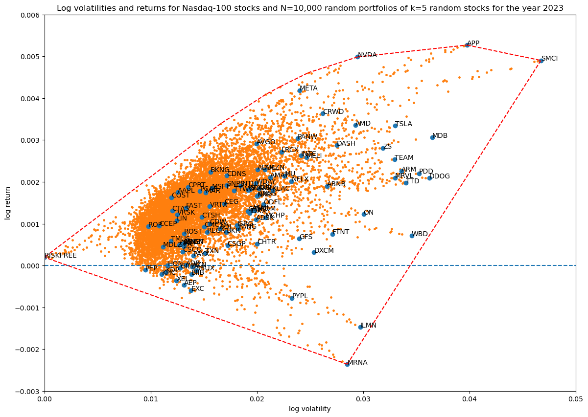
Running the alternative implementation:

random_portfolio = lambda num_tickers, portfolio_size:
    random_portfolio_implementation(num_tickers, portfolio_size, fix_last=True)
# same code as above

The difference is striking.

Note that throughout this article I use unit_random_angle_projection() from the previous article, which we saw is the best unit_random() implementation for exploring the log volatility—return space.

Coverage in log volatility—return space as a function of portfolio size

Finally, as in the first article, let's see how increasing the number of non-zero stocks in the portfolio weight vector increases coverage in log volatility—return space:

random_portfolio = lambda num_tickers, portfolio_size: random_portfolio_implementation(num_tickers, portfolio_size, fix_last=True)
unit_random = unit_random_angle_projection
num_simulations = 10_000
for portfolio_size in [2, 3, 5, 10, 50, 100]:
    title = f'...'
    portfolios = simulate_portfolios(df_r, portfolio_size, num_simulations)
    hulls[portfolio_size][num_simulations] = plot_portfolios(bare, portfolios, title)

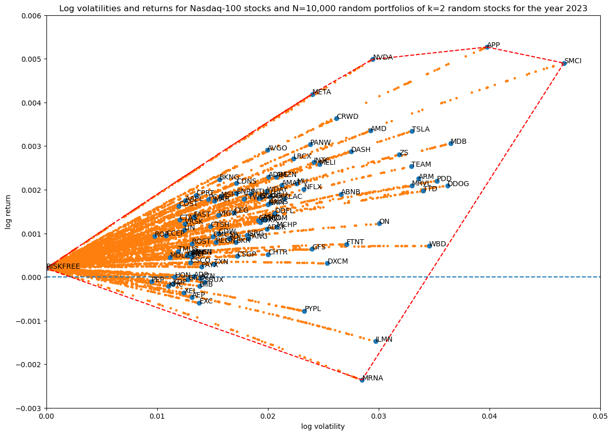
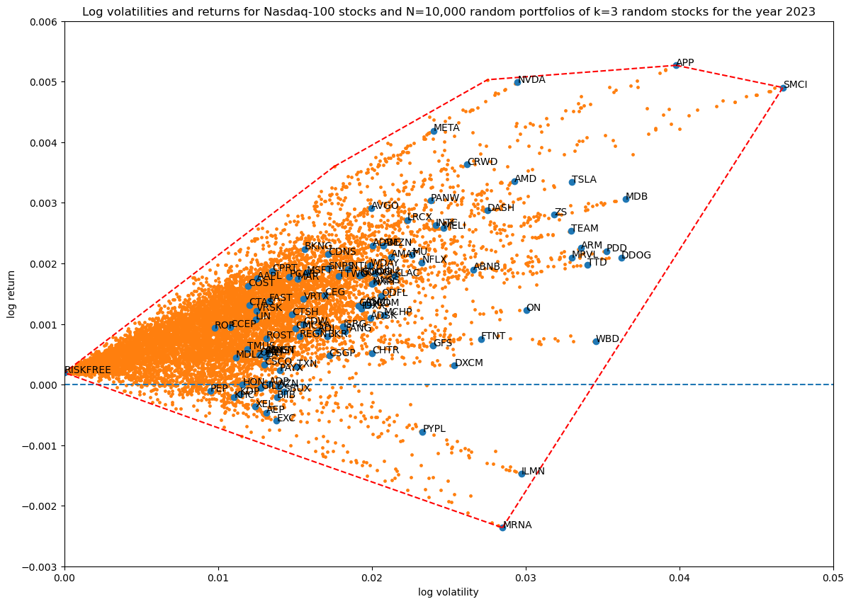
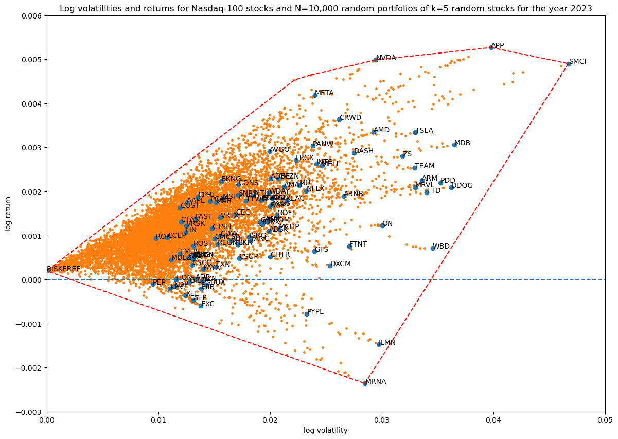
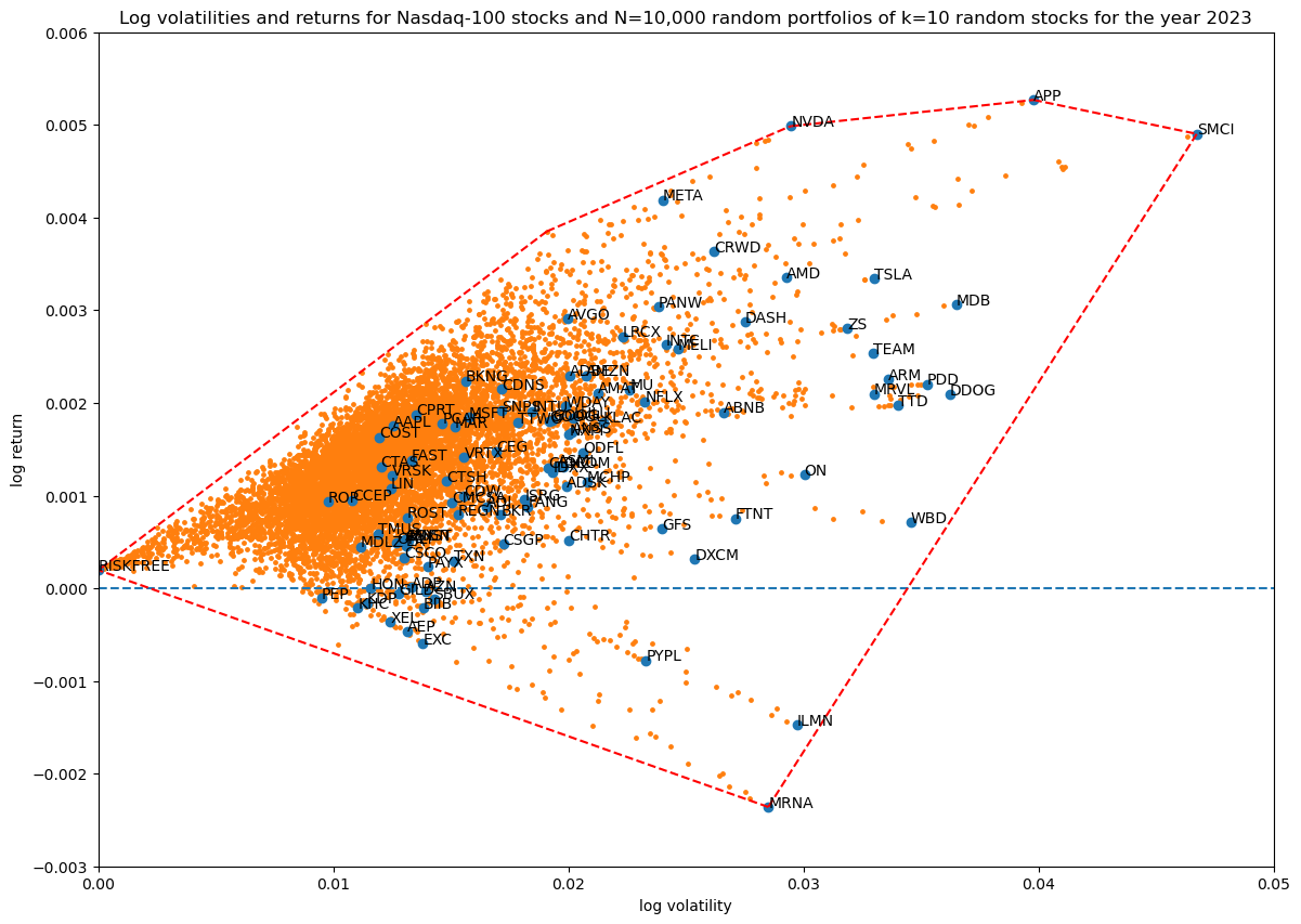
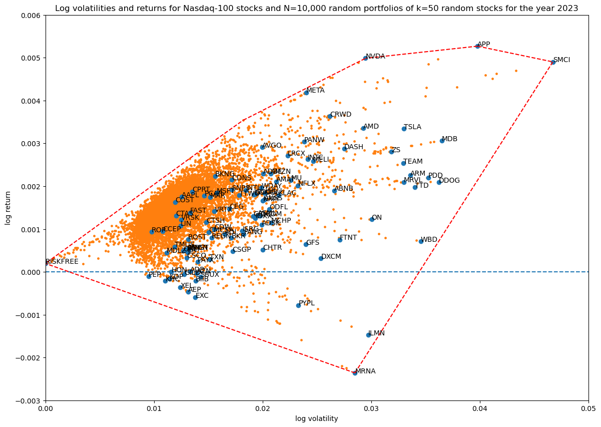
Progression of convex hulls:

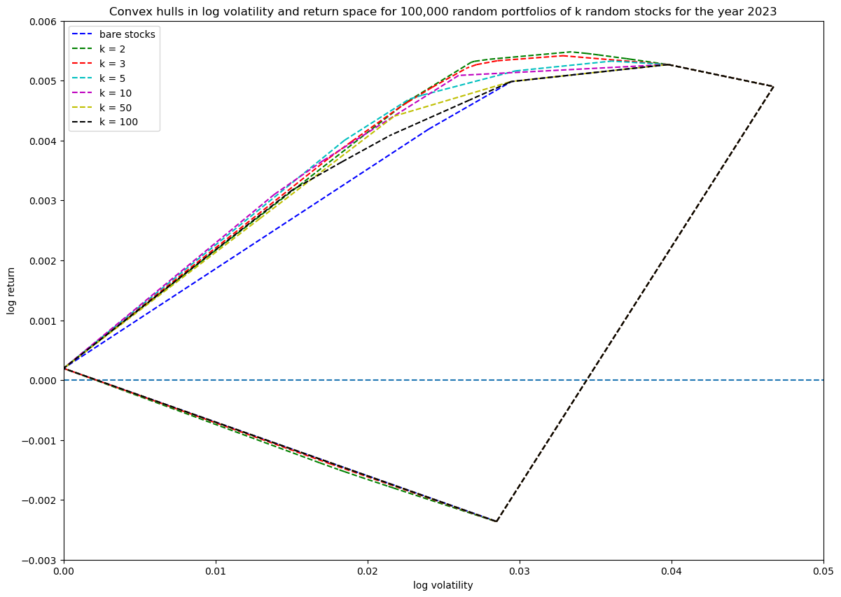
Overall, the effect of including the risk-free asset in our portfolio is visually clear: it extends the available volatility—return space in a convex way to the point defined by zero volatility and the fixed daily log-return of the risk-free asset.

Conclusion

Including the risk-free asset and running relatively simple Monte Carlo simulations already reproduces the overall shape of Markowitz's efficient frontier. In the next article, I will explicitly construct it using the traditional modern portfolio theory route of covariance matrix optimization.