Probabilistic spin glass - Part III

Introduction

In the previous articles (Part I, Part II), I looked at various properties of probabilistic spin glasses by simulating ensembles of many samples and computing various statistics, while in the case of entropy I computed probabilities directly. Here I will take a different route, and instead start with a starting grid, and let it evolve over "time" by changing spins one by one, and see how it behaves. The ipython notebook is on Github.

Evolution rule

Let's see what happens if we apply a dynamical probabilistic evolution operator to a probabilistic spin glass. The approach we will follow is simple:

1. Generate an initial grid per the (symmetrized) method described in the previous articles.
2. Pick a random (non-edge) spin, and given the four neighbours, pick a new alignment with the appropriate probability.

First, we have to arrive at the evolution probabilities: for a spin glass defined by $P(s=1 | n=1)=p$, what is the correct evolution probability given 4, already set neighbours? Instead of actually deriving the proability (which seems non-trivial to me), I cheat, and generate a large number of spin glasses and count frequencies to arrive at the probabilities. Since for 4 neighbours there are only $2^4=16$ possibilities, it's relatively easy to get good statistics.

def make_star_conditional(rows, cols, p0, p, num_simulations=1000):
    joint_frequencies, total = defaultdict(int), 0
    for simulation in range(num_simulations):
        pct = int((simulation / num_simulations) * 10000) / 100
        print(f'Computing conditionals for the {rows}x{cols} spin glass, progress {pct}% ', end='\r')
        sys.stdout.flush()
        grid = create_grid(rows, cols, p0, p)
        for i in range(1, rows-1):
            for j in range(1, cols-1):
                pattern = '%d%d%d%d%d' % (grid[i, j], grid[i, j-1], grid[i, j+1], grid[i-1, j], grid[i+1, j])
                joint_frequencies[pattern] += 1
                total += 1
    joint_probabilities = {} # joint_probabilities
    for pattern, freq in joint_frequencies.items():
        joint_probabilities[pattern] = freq/total
    return lambda up, down, left, right: ...

Visualization

Now we can run this probabilistic evolution, and on every steps_per_frame step, draw the frame on the screen:

def save_animation(filename, rows, cols, p0, starting_p, p, seconds=100, frames_per_second=5, steps_per_frame=6*1000):
    conditional_set_four_neighbours = make_star_conditional(rows, cols, p0, p)
    num_steps = seconds * frames_per_second * steps_per_frame
    grid, frames = create_grid(rows, cols, p0, starting_p), []
    for step in range(num_steps):
        if step % steps_per_frame == 0:
            frames.append(grid.copy())
        i, j = randint(1, rows-2), randint(1, cols-2)
        grid[i, j] = conditional_set_four_neighbours(grid[i, j-1], grid[i, j+1], grid[i-1, j], grid[i+1, j])
    fig = plt.figure()
    fig.suptitle(f'starting_p={starting_p:.2f}, p={p:0.2f}')
    im = plt.imshow(frames[0], cmap='Greys', vmin=0, vmax=1)
    plt.axis('off')
    def animate_func(i):
        im.set_array(frames[i])
        return [im]
    anim = animation.FuncAnimation(fig, animate_func,
        frames=seconds*frames_per_second,
        interval=1000/frames_per_second)
    anim.save(filename, fps=frames_per_second)

Previously, spin glasses had 4 parameters: rows, cols, p0, p. Here there's a fifth one, starting_p. This is in case we want the initial starting grid to be generated with a different p then in the evolution steps. This is interesting because we can check whether and how quickly the system forgets its initial configuration.

This is what a rows=50, cols=50, p0=0.5, starting_p=0.9, p=0.9 spin glass looks like:

And here is the same, but with starting_p=0.5, so it starts from random noise:

Note: the spins at the edges of the grid are not changed in the simulation.

The main takeaways:

1. On the first simulation, the overall pattern doesn't change much. This is because at p=0.9, if all 4 neighbours are the same spin alignment, the spin is very likely to align. So the spins that tend to change are the ones on the edges of the patterns, where at least 1 or 2 of the spins are not aligned.
2. On the second simulation with starting_p=0.5 we start out with a p=0.5 grid, which is just random noise. But then, very quickly, since we're evolving with the p=0.9 probabilities, out of the original randomnesss, a typical p=0.9 patterned grid forms, which then seemingly behaves like described in the previous point.

Visualizations of other parameters:

• rows=50, cols=50, p0=0.5, starting_p=0.5, p=0.5
• rows=50, cols=50, p0=0.5, starting_p=0.6, p=0.6
• rows=50, cols=50, p0=0.5, starting_p=0.7, p=0.7
• rows=50, cols=50, p0=0.5, starting_p=0.8, p=0.8
• rows=50, cols=50, p0=0.5, starting_p=0.9, p=0.9
• rows=50, cols=50, p0=0.5, starting_p=0.95, p=0.95
• rows=50, cols=50, p0=0.5, starting_p=0.975, p=0.975

Same, but starting from starting_p=0.5 noise:

• rows=50, cols=50, p0=0.5, starting_p=0.5, p=0.5
• rows=50, cols=50, p0=0.5, starting_p=0.5, p=0.6
• rows=50, cols=50, p0=0.5, starting_p=0.5, p=0.7
• rows=50, cols=50, p0=0.5, starting_p=0.5, p=0.8
• rows=50, cols=50, p0=0.5, starting_p=0.5, p=0.9
• rows=50, cols=50, p0=0.5, starting_p=0.5, p=0.95
• rows=50, cols=50, p0=0.5, starting_p=0.5, p=0.975

Convergence behaviour

We can check the convergence behaviour more systematically, ie. how quickly does the system forget the starting_p. Let's look at multiple trajectories, with different starting_ps, and let's use the majority fraction of spins that are aligned as the measure of order (so this is the y-axis):

def fraction(grid):
    r = np.sum(grid)/grid.size
    r = max(r, 1-r)
    return r

def get_trajectories(rows, cols, p0, starting_p, p, num_trajectories=3, seconds=100, frames_per_second = 5, steps_per_frame=6*1000):
    cache_key = str((rows, cols, p0, p))
    if cache_key not in conditional_set_four_neighbours_cached:
        conditional_set_four_neighbours_cached[cache_key] = make_star_conditional(rows, cols, p0, p)
    conditional_set_four_neighbours = conditional_set_four_neighbours_cached[cache_key]
    num_steps = seconds * frames_per_second * steps_per_frame
    trajectories = []
    starting_grid = create_grid(rows, cols, p0, starting_p)
    for t in range(num_trajectories):
        fs = []
        grid = starting_grid.copy()
        fs.append(fraction(grid))
        for step in range(num_steps):
            i, j = randint(1, rows-2), randint(1, cols-2)
            grid[i, j] = conditional_set_four_neighbours(grid[i, j-1], grid[i, j+1], grid[i-1, j], grid[i+1, j])
            if step % steps_per_frame == 0:
                fs.append(fraction(grid))
                pct = int((step / num_steps) * 10000) / 100
                print(f'Doing trajectory {t+1}/{num_trajectories} on the {rows}x{cols} spin glass, progress {pct}% ', end='\r')
                sys.stdout.flush()
        trajectories.append(fs)
    return trajectories

rows, cols, p0 = 50, 50, 0.5
mts = []
for p in [0.5, 0.6, 0.7, 0.8, 0.9, 0.95, 0.975]:
    for starting_p in [0.5, 0.6, 0.7, 0.8, 0.9, 0.95, 0.975]:
        trajectories = get_trajectories(
            rows=rows, cols=cols, p0=p0, starting_p=starting_p, p=p, num_trajectories=1)
        mts.append((p0, starting_p, p, trajectories[0]))

Yields:

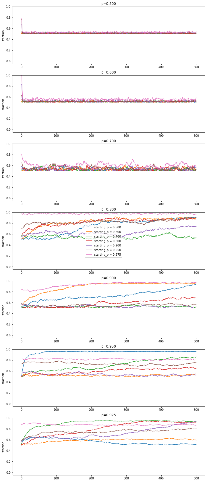
What this suggests is that it doesn't matter what the starting grid is, this initial condition is quickly washed out, and the grid behaves as if it always was running at its evoluationary p.

But why is the fraction so different in different simulation runs at higher p? To make sense of this, let's look at the fraction-curve from Part I again, but this time let's also plot the standard deviation, specifically for a $50 \times 50$ grids:

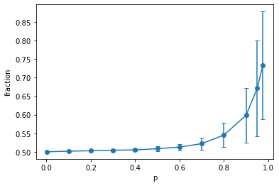
This is in agreement with what we see in the simulation runs: at p higher than 0.7, the standard deviation of the majority spin alignment is quite high, so there is a lot of deviation from the average fraction.

Conclusion

In the next and final piece I will make the system periodic and look at how behaviour changes with grid size.