The volatility of simple trading strategy returns

Introduction

In the previous post, I looked into the stability of volatilities of various securities, and found that there are significant year-over-year differences. The inspiration was to get a sense of the predictive power of frameworks such as Markowitz portfolio theory and CAPM, which rely on an accurate estimate of volatility (and returns) for portfolio choice.

In this post, I look at an alternative volatility measure, one more in line with the strategy of an imaginary trader. The thinking is simple: if the trader is following a strategy and of a sound mind (or is a soul-less algorithm), she doesn't care about short term price changes, only long-term outcomes of following the strategy. Of course, there is a big caveat: long-term outcomes are literally the sum of short-term daily changes. Still, I find it interesting to directly plot the returns (and volatility) of such imaginary traders.

The code is up on Github.

Trading algorithm

The algorithm is simple: buy the security on day 1, and exit early (sell) it the price goes up (take_profit) or down (stop_loss) by a certain amount. Otherwise, stick with it, but exit (sell) after a certain number of days (position_length), whatever the price:

 for daily_price in tail:
    if daily_price >= start_price * take_profit:
        final_price = start_price * take_profit
        break
    if daily_price <= start_price * stop_loss:
        final_price = start_price * stop_loss
        break
    final_price = daily_price

The returns are calculated by launching this strategy every day, and either exiting early, or running it until position_length days. This means that both the returs and variances/volatilities are highly correlated. The following function implements this strategy, prints out a histogram of daily returns, and year-over-year standard deviations:

def show_strategy_returns(df,  price_col='Adj Close', position_length=66, take_profit=1.5, stop_loss=0.5):
    df['Year'] = df.index.year
    years = list(df['Year'])
    sigmas = defaultdict(lambda: [])
    tickers = set([x[1] for x in list(df.columns) if x[1] != ''])
    for t in tickers:
        li = list(df[price_col][t])
        returns = []
        for i, start_price in enumerate(li):
            tail = li[i+1:i+1+position_length]
            if len(tail) < position_length: break
            for daily_price in tail:
                if daily_price >= start_price * take_profit:
                    final_price = start_price * take_profit
                    break
                if daily_price <= start_price * stop_loss:
                    final_price = start_price * stop_loss
                    break
                final_price = daily_price
            r = (final_price - start_price) / start_price
            returns.append(r)
        df_returns = pd.DataFrame(returns, columns=['returns'])
        df_returns.hist(bins=50, density=True)
        plt.title(t)
        # compute annual variance
        years = years[:len(returns)]
        sigmas[t] = [stdev([x[1] for x in zip(years, returns) if x[0] == year and x[1] == x[1]]) for year in set(years)]
    plt.clf()
    legend = []
    for t, s in sigmas.items():
        legend.append(t)
        plt.plot(sorted(set(years)), s, marker='o')
    plt.legend(legend)
    plt.xlabel('year')
    plt.ylabel(f'sigma of strategy')
    plt.ylim(0, )

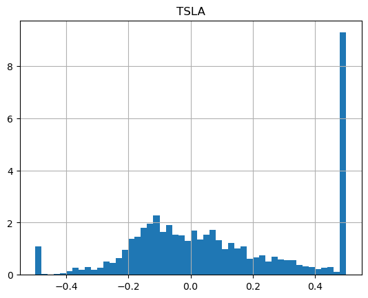
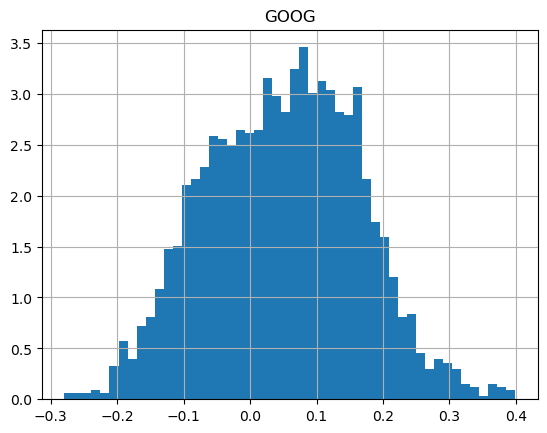
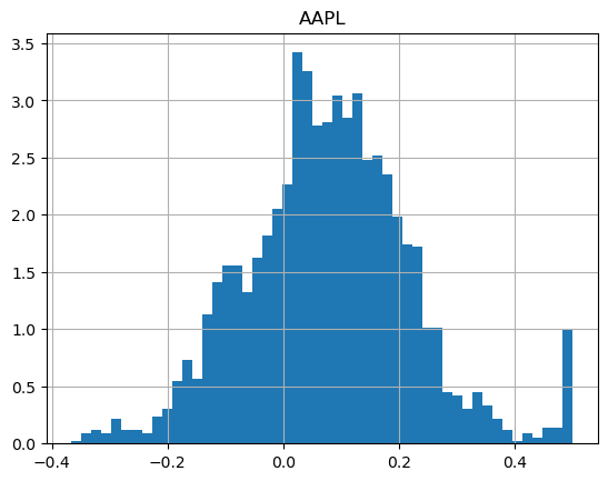
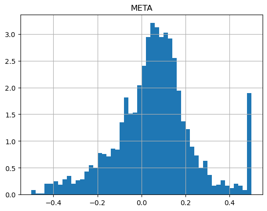
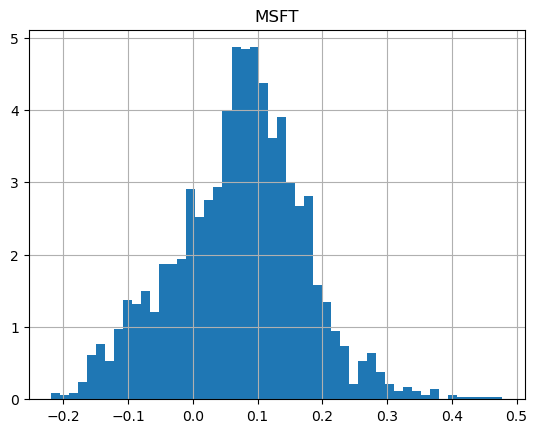
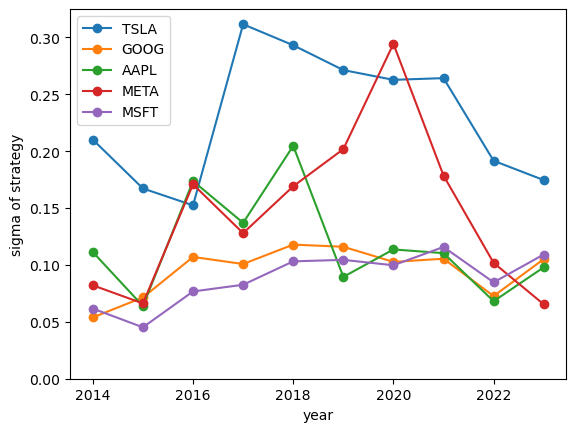
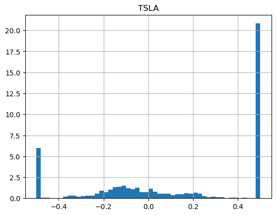
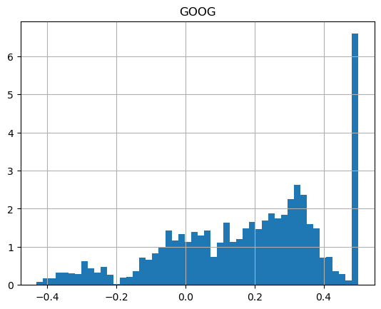
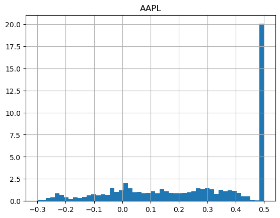
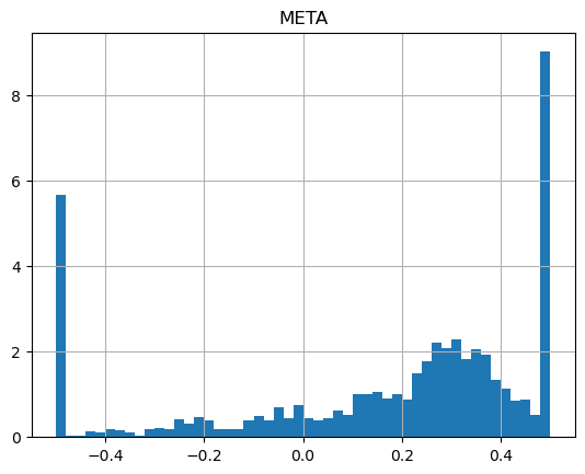
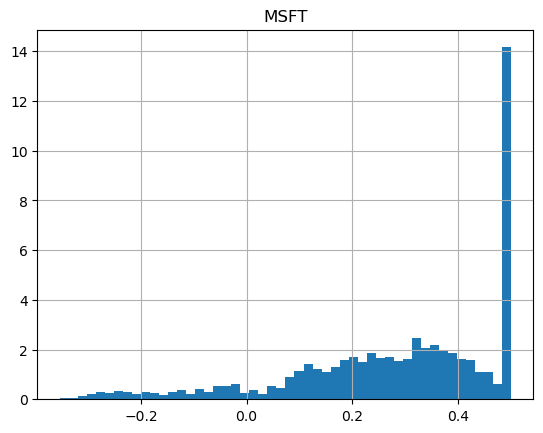
Let's run it for our tech stocks (Tesla, Google, Apple, Meta, Microsoft) in a greedy mode, where we want to make +50%, or stop loss at -50%, in a 3 month (66 trading days) window:

show_strategy_returns(df_tech, position_length=66, take_profit=1.5, stop_loss=0.5)

It's striking how different the shapes of the returns are:

How about if we run the same strategy, but with more patience, so we're willing to wait 1 whole year (252 trading days)?

show_strategy_returns(df_tech, position_length=252, take_profit=1.5, stop_loss=0.5)

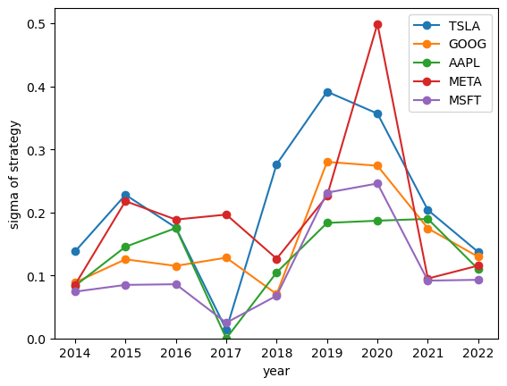
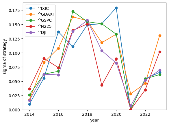
It's worth noting that in both cases, like with simple daily volatility measures, the year-over-year changes are significant. It seems hard to predict the upcoming year's volatility from previous years.

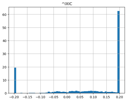
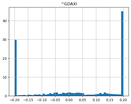
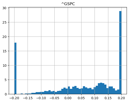
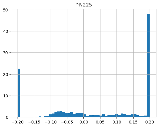
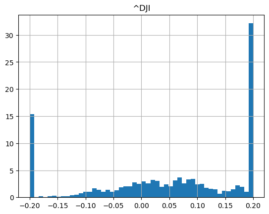
Let's run similar strategies on indices:

show_strategy_returns(df_indices, position_length=66, take_profit=1.2, stop_loss=0.8)

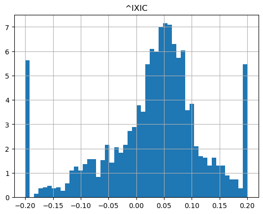
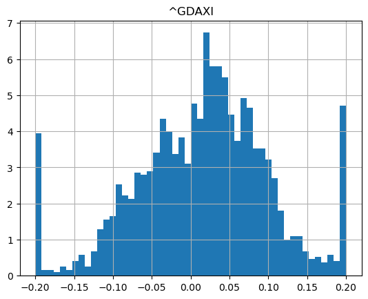
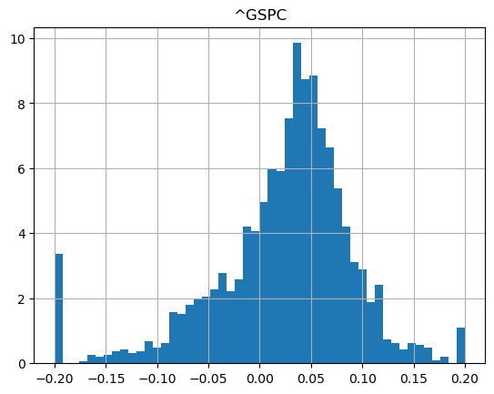
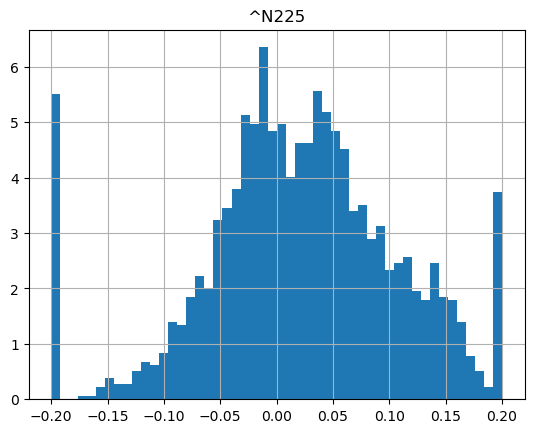
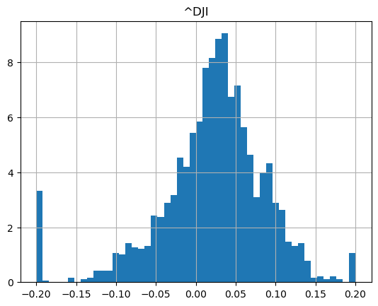
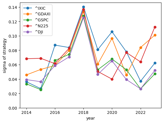
show_strategy_returns(df_indices, position_length=252, take_profit=1.2, stop_loss=0.8)

Conclusion

I will continue to investigate volatility measures, slowly working my ways to the Capital Asset Pricing Model.